10 Simulation

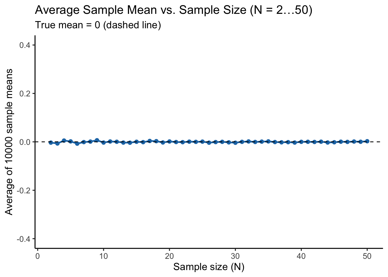
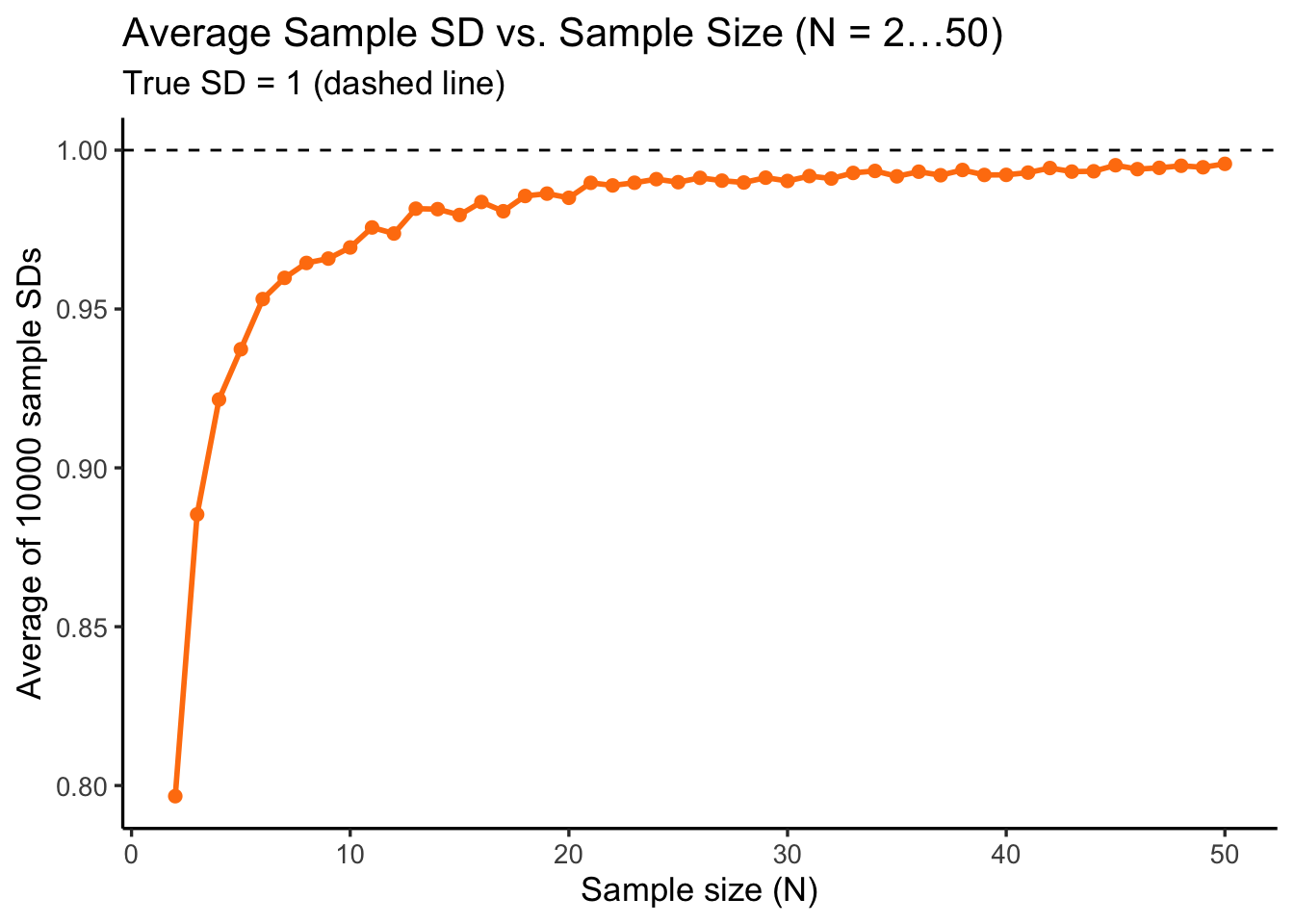
Here, we examine how sample size (N) affects estimates of the sample mean and sample standard deviation (SD). For each N = 2 to 50, draw 10000 samples from the standard normal distribution $\mathcal{N}(0, 1)$. Then, compute mean and SD for each sample. After that, calculate the average of these estimates to see how close they are to the true values (mean = 0, SD = 1).

set.seed(2025)

n_reps <- 10000
Ns     <- 2:50

# generate all combinations of sample size (N) and replicate number
results <- expand.grid(
  N      = Ns,
  replic = seq_len(n_reps)
) %>%
  arrange(N, replic)

# pre-calculate how many total simulations to run and 
# generate a vector of sample sizes for all rows
n_total <- nrow(results)
Ns_vec <- results$N

# system.time({
# generate all random samples in one go (total number of draws = sum of all Ns)
samples_all <- rnorm(sum(Ns_vec), mean = 0, sd = 1)

# assign an ID to each sample, to keep track of which row (i.e., which N) it belongs to
row_id <- rep(seq_along(Ns_vec), times = Ns_vec)

# split the generated samples by row
split_samples <- split(samples_all, row_id)

# compute sample mean and SD for each group
means <- sapply(split_samples, mean)
sds   <- sapply(split_samples, sd)
# })

# add results into the data frame
results$samp_mean <- means
results$samp_sd <- sds

# summarise the average sample mean and SD per sample size (N)
summary2 <- results %>%
  group_by(N) %>%
  summarize(
    avg_mean = mean(samp_mean),
    avg_sd = mean(samp_sd),
    .groups = "drop"
  )

# plot A: Average Sample Mean vs. N
p_avg_mean <- ggplot(summary2, aes(x = N, y = avg_mean)) +
  geom_point(color = "#1f77b4", size = 2) +
  geom_line(color = "#1f77b4", size = 1) +
  geom_hline(yintercept = 0, linetype = "dashed", color = "black") +
  labs(
    title = "Average Sample Mean vs. Sample Size (N = 2…50)",
    subtitle = "True mean = 0 (dashed line)",
    x = "Sample size (N)",
    y = "Average of 10000 sample means"
  ) +
  coord_cartesian(ylim = c(-0.4, 0.4)) +
  theme_classic(base_size = 13) +
  theme(
    panel.grid.minor = element_blank()
  )

# plot B: Average Sample SD vs. N
p_avg_sd <- ggplot(summary2, aes(x = N, y = avg_sd)) +
  geom_point(color = "#ff7f0e", size = 2) +
  geom_line(color = "#ff7f0e", size = 1) +
  geom_hline(yintercept = 1, linetype = "dashed", color = "black") +
  labs(
    title = "Average Sample SD vs. Sample Size (N = 2…50)",
    subtitle = "True SD = 1 (dashed line)",
    x = "Sample size (N)",
    y = "Average of 10000 sample SDs"
  ) +
  # coord_cartesian(ylim = c(-1.0, 1.0)) +
  theme_classic(base_size = 13) +
  theme(
    panel.grid.minor = element_blank()
  )

# display the two plots
p_avg_mean

p_avg_sd

For small sample sizes, sample variance and standard deviation tend to be biased, as shown in the bottom plot, the average sample SD is clearly lower than 1 when N is small. Once N exceeds approximately 20, the average sample SD (and variance) gets much closer to 1, and the bias becomes negligible.

11 References

Cleasby IR, Burke T, Schroeder J, Nakagawa S. (2011) Food supplements increase adult tarsus length, but not growth rate, in an island population of house sparrows (Passer domesticus). BMC Research Notes. 4:1-1. doi: 10.1186/1756-0500-4-431
Drummond H, Rodriguez C, Ortega S. (2025). Long-Term Insights into Who Benefits from Brood Reduction. Behavioral Ecology. doi: 10.1093/beheco/araf050
Mizuno A, Soma M. (2023) Pre-existing visual preference for white dot patterns in estrildid finches: a comparative study of a multi-species experiment. Royal Society Open Science. 10:231057. doi: 10.1098/rsos.231057
Lundgren EJ, Ramp D, Middleton OS, Wooster EI, Kusch E, Balisi M, Ripple WJ, Hasselerharm CD, Sanchez JN, Mills M, Wallach AD. (2022) A novel trophic cascade between cougars and feral donkeys shapes desert wetlands. Journal of Animal Ecology. 91:2348-57. doi: 10.1111/1365-2656.13766
Aki Vehtari, Andrew Gelman, Daniel Simpson, Bob Carpenter, Paul-Christian Bürkner (2021). Rank-Normalization, Folding, and Localization: An Improved Rhat for Assessing Convergence of MCMC (with Discussion). Bayesian Analysis. 16:667-718. doi: 10.1214/20-BA1221

12 Information about `R` session

This section shows the current R session information, including R version, platform, and loaded packages.

sessionInfo()

R version 4.4.2 (2024-10-31)
Platform: aarch64-apple-darwin20
Running under: macOS Sequoia 15.6.1

Matrix products: default
BLAS:   /Library/Frameworks/R.framework/Versions/4.4-arm64/Resources/lib/libRblas.0.dylib 
LAPACK: /Library/Frameworks/R.framework/Versions/4.4-arm64/Resources/lib/libRlapack.dylib;  LAPACK version 3.12.0

locale:
[1] en_US.UTF-8/en_US.UTF-8/en_US.UTF-8/C/en_US.UTF-8/en_US.UTF-8

time zone: America/Edmonton
tzcode source: internal

attached base packages:
[1] parallel  stats     graphics  grDevices utils     datasets  methods  
[8] base     

other attached packages:
 [1] knitr_1.50          kableExtra_1.4.0    here_1.0.1         
 [4] gt_1.0.0            tidybayes_3.0.7     patchwork_1.3.1    
 [7] bayesplot_1.13.0    MuMIn_1.48.11       loo_2.8.0          
[10] DHARMa_0.4.7        TreeTools_1.14.0    rstan_2.32.7       
[13] StanHeaders_2.32.10 phytools_2.4-4      maps_3.4.3         
[16] glmmTMB_1.1.11      emmeans_1.11.1      cmdstanr_0.9.0.9000
[19] brms_2.23.0         Rcpp_1.1.0          arm_1.14-4         
[22] lme4_1.1-37         Matrix_1.7-3        MASS_7.3-65        
[25] ape_5.8-1           broom.mixed_0.2.9.6 broom_1.0.8        
[28] lubridate_1.9.4     forcats_1.0.0       stringr_1.5.1      
[31] purrr_1.0.4         readr_2.1.5         tidyr_1.3.1        
[34] ggplot2_3.5.2       tidyverse_2.0.0     tibble_3.3.0       
[37] dplyr_1.1.4        

loaded via a namespace (and not attached):
  [1] RColorBrewer_1.1-3      tensorA_0.36.2.1        rstudioapi_0.17.1      
  [4] jsonlite_2.0.0          magrittr_2.0.3          TH.data_1.1-3          
  [7] estimability_1.5.1      farver_2.1.2            nloptr_2.2.1           
 [10] rmarkdown_2.29          vctrs_0.6.5             minqa_1.2.8            
 [13] RCurl_1.98-1.17         htmltools_0.5.8.1       distributional_0.5.0   
 [16] curl_6.4.0              DEoptim_2.2-8           parallelly_1.45.0      
 [19] htmlwidgets_1.6.4       sandwich_3.1-1          zoo_1.8-14             
 [22] TMB_1.9.17              igraph_2.1.4            lifecycle_1.0.4        
 [25] iterators_1.0.14        pkgconfig_2.0.3         R6_2.6.1               
 [28] fastmap_1.2.0           rbibutils_2.3           future_1.58.0          
 [31] digest_0.6.37           numDeriv_2016.8-1.1     colorspace_2.1-1       
 [34] furrr_0.3.1             ps_1.9.1                rprojroot_2.0.4        
 [37] textshaping_1.0.1       labeling_0.4.3          clusterGeneration_1.3.8
 [40] timechange_0.3.0        abind_1.4-8             mgcv_1.9-3             
 [43] compiler_4.4.2          bit64_4.6.0-1           withr_3.0.2            
 [46] doParallel_1.0.17       backports_1.5.0         inline_0.3.21          
 [49] optimParallel_1.0-2     QuickJSR_1.8.0          pkgbuild_1.4.8         
 [52] R.utils_2.13.0          scatterplot3d_0.3-44    tools_4.4.2            
 [55] R.oo_1.27.1             glue_1.8.0              quadprog_1.5-8         
 [58] nlme_3.1-168            R.cache_0.17.0          grid_4.4.2             
 [61] checkmate_2.3.2         PlotTools_0.3.1         generics_0.1.4         
 [64] gtable_0.3.6            tzdb_0.5.0              R.methodsS3_1.8.2      
 [67] hms_1.1.3               xml2_1.3.8              ggdist_3.3.3           
 [70] foreach_1.5.2           pillar_1.11.0           posterior_1.6.1        
 [73] splines_4.4.2           lattice_0.22-7          bit_4.6.0              
 [76] survival_3.8-3          tidyselect_1.2.1        arrayhelpers_1.1-0     
 [79] reformulas_0.4.1        gridExtra_2.3           V8_6.0.4               
 [82] svglite_2.2.1           stats4_4.4.2            xfun_0.52              
 [85] expm_1.0-0              bridgesampling_1.1-2    matrixStats_1.5.0      
 [88] stringi_1.8.7           yaml_2.3.10             pacman_0.5.1           
 [91] boot_1.3-31             evaluate_1.0.4          codetools_0.2-20       
 [94] cli_3.6.5               RcppParallel_5.1.10     systemfonts_1.2.3      
 [97] xtable_1.8-4            Rdpack_2.6.4            processx_3.8.6         
[100] globals_0.18.0          coda_0.19-4.1           svUnit_1.0.6           
[103] rstantools_2.4.0        bitops_1.0-9            Brobdingnag_1.2-9      
[106] listenv_0.9.1           phangorn_2.12.1         viridisLite_0.4.2      
[109] mvtnorm_1.3-3           scales_1.4.0            combinat_0.0-8         
[112] rlang_1.1.6             fastmatch_1.1-6         multcomp_1.4-28        
[115] mnormt_2.1.1

--- title: "Simulation" --- ```{r} #| label: load_packages #| echo: false # Load required packages pacman::p_load( ## data manipulation dplyr, tibble, tidyverse, broom, broom.mixed, ## model fitting ape, arm, brms, broom.mixed, cmdstanr, emmeans, glmmTMB, MASS, phytools, rstan, TreeTools, ## model checking and evaluation DHARMa, loo, MuMIn, parallel, ## visualisation bayesplot, ggplot2, patchwork, tidybayes, ## reporting and utilities gt, here, kableExtra, knitr ) ``` Here, we examine how sample size (N) affects estimates of the sample mean and sample standard deviation (SD). For each N = 2 to 50, draw 10000 samples from the standard normal distribution $\mathcal{N}(0, 1)$. Then, compute mean and SD for each sample. After that, calculate the average of these estimates to see how close they are to the true values (mean = 0, SD = 1). ```{r} #| echo: false #| eval: false # # 1. simulation settings # set.seed(2025) # n_reps <- 10000 # replicates per N # Ns <- 2:50 # N = 2, 3, 4, …, 50 # # 2. simulate draws and compute sample mean & SD for each combination of N and replicate # ## create a data frame with all combinations of N and replication number # ## in this case, for N = 2 to 50 and 10000 replicates per N, this create 49*1000 = 49000 rows # results <- expand.grid( # N = Ns, # replic = seq_len(n_reps) # replicate number from 1 to 1000 # ) %>% # arrange(N, replic) %>% # sort by N and replicate number # mutate( # samp_mean = NA_real_, # placeholder for sample mean # samp_sd = NA_real_ # placeholder for sample SD # ) # # loop through each N and compute sample mean and SD # for (i in seq_len(nrow(results))) { # N <- results$N[i] # extract the sample size for this row # x <- rnorm(N, mean = 0, sd = 1) # simulate N random values from N(0,1) # results$samp_mean[i] <- mean(x) # compute and store the sample mean # results$samp_sd[i] <- sd(x) # compute and store the sample SD # } # # 3. for each sample size N, compute the average sample mean and average sample SD across all replicates # summary2 <- results %>% # group_by(N) %>% # summarize( # avg_mean = mean(samp_mean), # avg_sd = mean(samp_sd) # ) %>% # ungroup() # # 4. plot A: Average Sample Mean vs. N # p_avg_mean <- ggplot(summary2, aes(x = N, y = avg_mean)) + # geom_point(color = "#1f77b4", size = 2) + # geom_line(color = "#1f77b4", size = 1) + # geom_hline(yintercept = 0, linetype = "dashed", color = "black") + # labs( # title = "Average Sample Mean vs. Sample Size (N = 2…50)", # subtitle = "True mean = 0 (dashed line)", # x = "Sample size (N)", # y = "Average of 10000 sample means" # ) + # theme_classic(base_size = 13) + # theme( # panel.grid.minor = element_blank() # ) # # 5. plot B: Average Sample SD vs. N # p_avg_sd <- ggplot(summary2, aes(x = N, y = avg_sd)) + # geom_point(color = "#ff7f0e", size = 2) + # geom_line(color = "#ff7f0e", size = 1) + # geom_hline(yintercept = 1, linetype = "dashed", color = "black") + # labs( # title = "Average Sample SD vs. Sample Size (N = 2…50)", # subtitle = "True SD = 1 (dashed line)", # x = "Sample size (N)", # y = "Average of 10000 sample SDs" # ) + # theme_classic(base_size = 13) + # theme( # panel.grid.minor = element_blank() # ) # # 6. display the two plots # p_avg_mean # p_avg_sd ``` ```{r} set.seed(2025) n_reps <- 10000 Ns <- 2:50 # generate all combinations of sample size (N) and replicate number results <- expand.grid( N = Ns, replic = seq_len(n_reps) ) %>% arrange(N, replic) # pre-calculate how many total simulations to run and # generate a vector of sample sizes for all rows n_total <- nrow(results) Ns_vec <- results$N # system.time({ # generate all random samples in one go (total number of draws = sum of all Ns) samples_all <- rnorm(sum(Ns_vec), mean = 0, sd = 1) # assign an ID to each sample, to keep track of which row (i.e., which N) it belongs to row_id <- rep(seq_along(Ns_vec), times = Ns_vec) # split the generated samples by row split_samples <- split(samples_all, row_id) # compute sample mean and SD for each group means <- sapply(split_samples, mean) sds <- sapply(split_samples, sd) # }) # add results into the data frame results$samp_mean <- means results$samp_sd <- sds # summarise the average sample mean and SD per sample size (N) summary2 <- results %>% group_by(N) %>% summarize( avg_mean = mean(samp_mean), avg_sd = mean(samp_sd), .groups = "drop" ) # plot A: Average Sample Mean vs. N p_avg_mean <- ggplot(summary2, aes(x = N, y = avg_mean)) + geom_point(color = "#1f77b4", size = 2) + geom_line(color = "#1f77b4", size = 1) + geom_hline(yintercept = 0, linetype = "dashed", color = "black") + labs( title = "Average Sample Mean vs. Sample Size (N = 2…50)", subtitle = "True mean = 0 (dashed line)", x = "Sample size (N)", y = "Average of 10000 sample means" ) + coord_cartesian(ylim = c(-0.4, 0.4)) + theme_classic(base_size = 13) + theme( panel.grid.minor = element_blank() ) # plot B: Average Sample SD vs. N p_avg_sd <- ggplot(summary2, aes(x = N, y = avg_sd)) + geom_point(color = "#ff7f0e", size = 2) + geom_line(color = "#ff7f0e", size = 1) + geom_hline(yintercept = 1, linetype = "dashed", color = "black") + labs( title = "Average Sample SD vs. Sample Size (N = 2…50)", subtitle = "True SD = 1 (dashed line)", x = "Sample size (N)", y = "Average of 10000 sample SDs" ) + # coord_cartesian(ylim = c(-1.0, 1.0)) + theme_classic(base_size = 13) + theme( panel.grid.minor = element_blank() ) # display the two plots p_avg_mean p_avg_sd ``` For small sample sizes, sample variance and standard deviation tend to be biased, as shown in the bottom plot, the average sample SD is clearly lower than 1 when N is small. Once N exceeds approximately 20, the average sample SD (and variance) gets much closer to 1, and the bias becomes negligible. # References - Cleasby IR, Burke T, Schroeder J, Nakagawa S. (2011) Food supplements increase adult tarsus length, but not growth rate, in an island population of house sparrows (Passer domesticus). *BMC Research Notes*. 4:1-1. doi: 10.1186/1756-0500-4-431 - Drummond H, Rodriguez C, Ortega S. (2025). Long-Term Insights into Who Benefits from Brood Reduction. *Behavioral Ecology*. doi: 10.1093/beheco/araf050 - Mizuno A, Soma M. (2023) Pre-existing visual preference for white dot patterns in estrildid finches: a comparative study of a multi-species experiment. *Royal Society Open Science*. 10:231057. doi: 10.1098/rsos.231057 - Lundgren EJ, Ramp D, Middleton OS, Wooster EI, Kusch E, Balisi M, Ripple WJ, Hasselerharm CD, Sanchez JN, Mills M, Wallach AD. (2022) A novel trophic cascade between cougars and feral donkeys shapes desert wetlands. *Journal of Animal Ecology*. 91:2348-57. doi: 10.1111/1365-2656.13766 - Aki Vehtari, Andrew Gelman, Daniel Simpson, Bob Carpenter, Paul-Christian Bürkner (2021). Rank-Normalization, Folding, and Localization: An Improved Rhat for Assessing Convergence of MCMC (with Discussion). *Bayesian Analysis*. 16:667-718. doi: 10.1214/20-BA1221 # Information about `R` session This section shows the current `R` session information, including `R` version, platform, and loaded packages. ```{r} sessionInfo() ```

11 References

12 Information about R session

12 Information about `R` session