dat <- read_csv(here("data","SMI_Drummond_et_al_2025.csv")) %>%subset(REDUCTION == 0)

dat<- dat%>%
  dplyr::select(-TIME, -HATCHING_DATE,-REDUCTION,-RING) %>%
  mutate(SMI = as.numeric(SMI),# Scaled mass index
         lnSMI=log(SMI),
         NEST = as.factor(NEST),
         WORKYEAR = as.factor(WORKYEAR),
RANK = factor(RANK, levels = c("1", "2")))4 Double-hierarchical location-scale model (Model 3)
Following up on the previous example analyzing the scaled mass index (SMI) at fledgling Drummond et al(2025), we now extend our approach by fitting a double-hierarchical Gaussian location-scale model. This extends Model 2 by introducing nest identity as a correlated random effect in both the location (mean) and scale (variance) components. This extension allows us to examine not only how average log(SMI) and its variability differ across nests, but also whether these two forms of nest-level variation are correlated. The main distinction between Model 2 and Model 3 lies in how they handle variation. Model 2 includes random effects only for the mean, assuming constant variance across groups. In contrast, Model 3 accounts for group-level variability by including random effects in both the mean and the variance components. This makes Model 3 particularly useful when:
Group-level variability (heteroscedasticity) is present
There may be a correlation between group-level means and variances (e.g., nests with higher average SMI also show more variability)
Both the average and variability are biologically meaningful or expected to vary across groups
By modeling variation explicitly, Model 3 can yield better fit and more nuanced inference, especially in ecological or evolutionary contexts where both central tendencies and dispersion carry important signals.
4.1 Dataset overview
We use the same dataset as in Model 2, but extend the location-scale framework by moving from Model 2 to Model 3, a double-hierarchical location-scale model. This extension allows us to model group-level variation in both the mean (location) and the variance (scale), as well as their potential correlation.
4.1.1 Question
Variation between and within nests Do nests with generally healthier (heavier) chicks also tend to have chicks that are more similar in their body condition?
4.2 Run models and interpret results
In this section, we compare Model 1 and Model 3 using the brms package, since glmmTMB does not support estimating correlations between random effects in the location and scale components. Model 3 - the double-hierarchical location-scale model - extends Model 2 by incorporating random effects for NEST_ID in both the mean and the variability of SMI. Crucially, it also estimates the correlation between these nest-level effects. For instance, a positive correlation would indicate that nests with higher average SMI also exhibit greater variability in SMI.
m3 <- bf(log(SMI) ~ 1 + RANK+ (1|q|NEST) + (1|WORKYEAR),
         sigma~ 1 + RANK + (1|q|NEST) + (1|WORKYEAR))
prior3<-default_prior(m3,data = dat,family = gaussian())

fit3 <- brm(
  m3,
  prior= prior3,
  data = dat,
  family = gaussian(),
  iter = 6000,
  warmup = 1000,
  chains = 4,
  cores=4,
  backend = "cmdstanr",
  control = list(
    adapt_delta = 0.99,
    max_treedepth = 15
    ),
  seed = 123,
  refresh = 500)
Family: gaussian
Links: mu = identity; sigma = log
Formula: log(SMI) ~ (1 | q | NEST) + (1 | WORKYEAR) + RANK
sigma ~ (1 | q | NEST) + (1 | WORKYEAR) + RANK
Data: dat (Number of observations: 4737)
Draws: 4 chains, each with iter = 6000; warmup = 1000; thin = 1;
total post-warmup draws = 20000
Multilevel Hyperparameters:
~NEST (Number of levels: 2873)
Estimate Est.Error l-95% CI u-95% CI Rhat
sd(Intercept) 0.05 0.00 0.04 0.05 1.00
sd(sigma_Intercept) 0.36 0.02 0.32 0.40 1.00
cor(Intercept,sigma_Intercept) -0.46 0.07 -0.58 -0.33 1.00
Bulk_ESS Tail_ESS
sd(Intercept) 3596 7826
sd(sigma_Intercept) 4668 9783
cor(Intercept,sigma_Intercept) 3805 7596
~WORKYEAR (Number of levels: 24)
Estimate Est.Error l-95% CI u-95% CI Rhat Bulk_ESS Tail_ESS
sd(Intercept) 0.10 0.02 0.07 0.14 1.00 5949 10071
sd(sigma_Intercept) 0.28 0.06 0.18 0.41 1.00 8421 12541
Regression Coefficients:
Estimate Est.Error l-95% CI u-95% CI Rhat Bulk_ESS Tail_ESS
Intercept 7.36 0.02 7.32 7.40 1.00 3428 6959
sigma_Intercept -2.52 0.07 -2.65 -2.38 1.00 5030 8529
RANK2 -0.01 0.00 -0.02 -0.01 1.00 24251 17886
sigma_RANK2 0.13 0.03 0.07 0.19 1.00 19128 15170
Draws were sampled using sample(hmc). For each parameter, Bulk_ESS
and Tail_ESS are effective sample size measures, and Rhat is the potential
scale reduction factor on split chains (at convergence, Rhat = 1).We compare the double-hierarchical location-scale model (Model 3) with the previous location-only model (Model 1) to examine whether the added complexity of Model 3 leads to a better fit to the data.
f1loo <- loo::loo(fit1)
f3loo <- loo::loo(fit3)

#Model comparison
fc2 <- loo::loo_compare(f1loo, f3loo)
fc2
#  elpd_diff se_diff
# fit3    0.0       0.0
# fit1 -357.2      37.4
The impact of including random effects in the scale component becomes clear when comparing the results of Model 1 with those of the double-hierarchical location-scale model (Model 3).
m3_draws<-fit3 %>%
  tidybayes::epred_draws(newdata = expand.grid(
    RANK = unique(dat$RANK)
  ), re_formula = NA, dpar =TRUE)


plot_lm3 <- ggplot(m3_draws, aes(x = factor(RANK), y = .epred,fill = factor(RANK))) +
  geom_violin(alpha = 0.5, show.legend = FALSE)+
  stat_pointinterval(show.legend = FALSE) +
  labs(
    title = "Location",
    x = "Hatching order",
    y = "log(SMI)"
  ) +
  theme_classic() + scale_y_continuous(breaks = seq(7.2,7.5,0.05),limits = c(7.2, 7.5))


plot_sm3 <- ggplot(m3_draws, aes(x = factor(RANK), y = sigma,fill = factor(RANK))) +
geom_violin(alpha = 0.5, show.legend = FALSE)+
  stat_pointinterval(show.legend = FALSE) +
  labs(
    title = "Scale",
    x = "Hatching order",
    y = "log(Standard Deviation)"
  ) +
  theme_classic() + scale_y_continuous(breaks = seq(0.04,0.12,0.01),limits = c(0.04, 0.12))


correlation_draws <- fit3 %>%
  spread_draws(cor_NEST__Intercept__sigma_Intercept)


corr_plot<-ggplot(data=correlation_draws,aes(x = cor_NEST__Intercept__sigma_Intercept)) +
   stat_halfeye() +
  labs(
    title = "Correlation between location and the scale intercepts in the NEST group",
    x = "cor(Intercept, sigma_Intercept)",
    y = "Density"
  ) +
  theme_classic()


combinded_plot<-((plot_lm3 + plot_sm3)/corr_plot)&
  theme(
    panel.grid.major = element_blank(),
    panel.grid.minor = element_blank()
  )
combinded_plot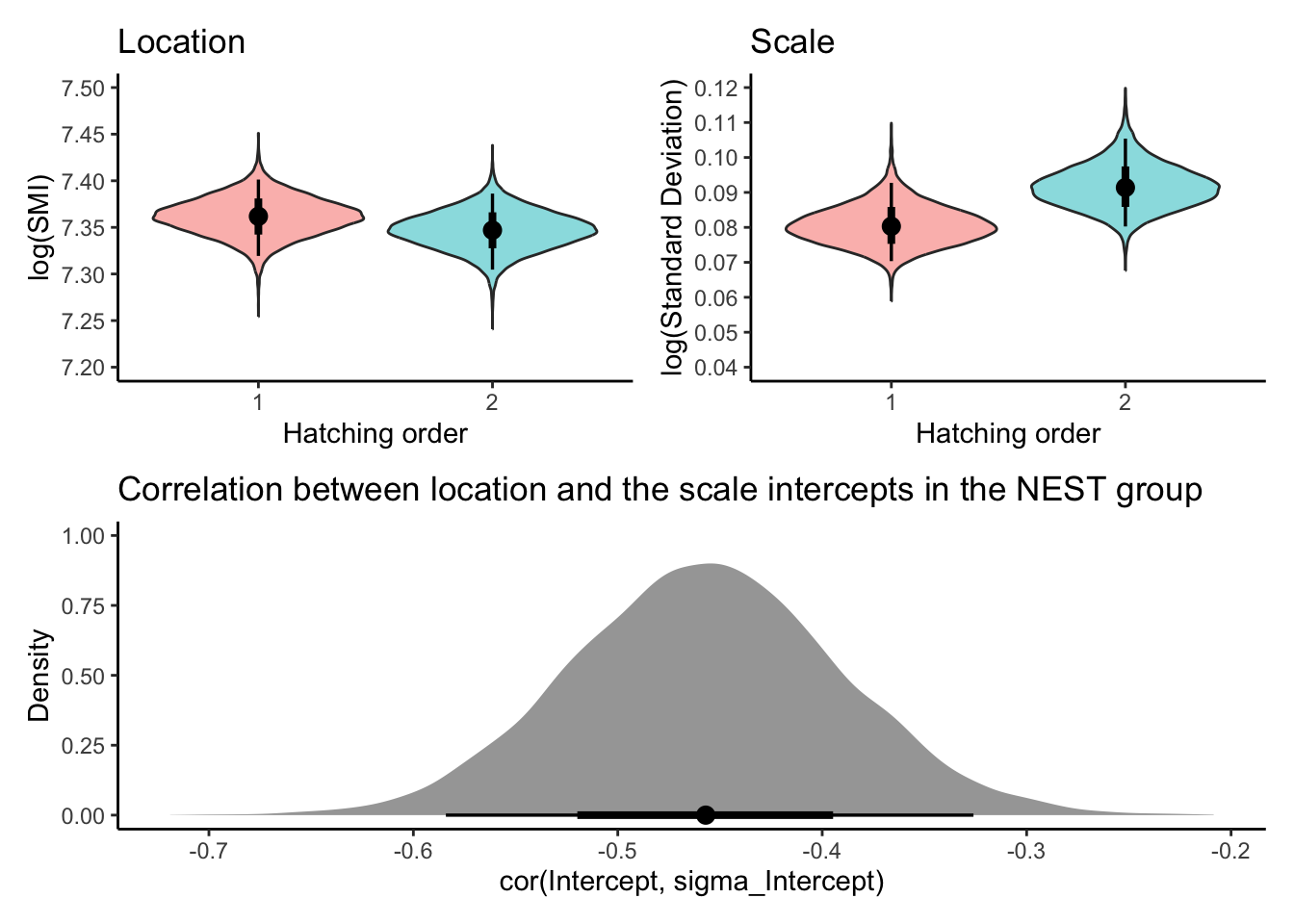
4.2.1 Comparison of location-only model and location-scale model
The model comparison results indicate that the double-hierarchical location-scale model (Model 3) is the most supported by the data, as it has the lowest LOO (Leave-One-Out Cross-Validation) information criterion value. This suggests that this model provides the best fit to the data while accounting for both the average differences in body condition and the variability in body condition between first and second-hatched chicks.
4.2.2 Interpretation of location-scale model :
Scale (dispersion) random effects:
There is notable variation in body condition within nests (\(\sigma_{[\text{Nest\_ID}]}^{(s)}\) = 0.37, 95% CI [0.316, 0.399]). This indicates that some nests consistently produce chicks with more consistent body conditions than others.
The consistency of chick body conditions varies notably across work years (\(\sigma_{[\text{Year}]}^{(s)}\) = 0.277, 95% CI [0.183, 0.411]), implying some years yield chicks with more consistent body conditions than others.
Correlation between location and scale random effects:
- The correlation between the nest-specific random effects for the average body condition and the variability in body condition is negative (\(\rho_{[\text{Nest\_ID}]}\) = -0.457, 95% CI [-0.584, -0.326]). This suggests that nests with higher average body conditions tend to produce chicks with more consistent body condition values (less dispersion).
4.3 Conclusion
Do nests with generally healthier (heavier) chicks also tend to have chicks that are more similar in their body condition?
Answer: Yes, there’s a tendency for nests with higher average chick body condition to also exhibit greater consistency among their chicks’ body conditions. This is supported by a negative correlation between nest-specific average body condition and its variability.
Note
Modeling Correlated Random Effects with brms vs. glmmTMB
This specific hierarchical model can be fit using brms but not with glmmTMB due to a key difference in their capabilities.
The model has two parts: one predicting the mean (mu) of the outcome and another predicting its variability (sigma). For each grouping factor (e.g., NEST), the model estimates a random effect for both the mean and the variability.
The core issue is that glmmTMB cannot estimate the correlation between these two different random effects. It is forced to assume that a group’s effect on the mean is completely unrelated to its effect on the variability. brms, being a more flexible Bayesian tool, can estimate this relationship directly from the data.
Therefore, if your hypothesis involves a potential link between the random effects for different parts of your model (e.g., “do nests with higher average SMI also have less variable SMI?”), you must use a package like brms that can model this covariance.