3 Adding random effects in the location part only (model 2)

Model 2 is a location-scale model with random effects in the location part only. This allows us to account for individual-level variation in the mean response while still modeling the dispersion separately.

3.1 Dataset overview

This dataset comes from Drummond et al (2025), which examined the benefits of brood reduction in the blue-footed booby (Sula nebouxii).Focusing on two-chick broods, the research explored whether the death of one chick (brood reduction) primarily benefits the surviving sibling (via increased resource acquisition) or the parents (by lessening parental investment). In this species, older chicks establish a strong dominance hierarchy over their younger siblings. Under stressful environmental conditions, this often results in the death of the second-hatched chick, with parental intervention being extremely rare.

For this tutorial, we will specifically examine data from two-chick broods where both chicks survived to fledgling. Our analysis will focus on how hatching order influences the body condition of chicks at fledgling.

3.1.1 Questions

Do first hatched chicks have a higher body mass than second-hatched chicks?
Does the variability in body mass differ between first and second-hatched chicks?

3.1.2 Variables included

SMI: Scaled Mass Index, a measure that accounts for body mass relative to size
RANK: The order in which chicks hatched (1 for first-hatched, 2 for second-hatched)
NEST_ID: Identifier for the nest where the chicks were raised
YEAR: The year in which the chicks were born

3.2 Visualise the dataset

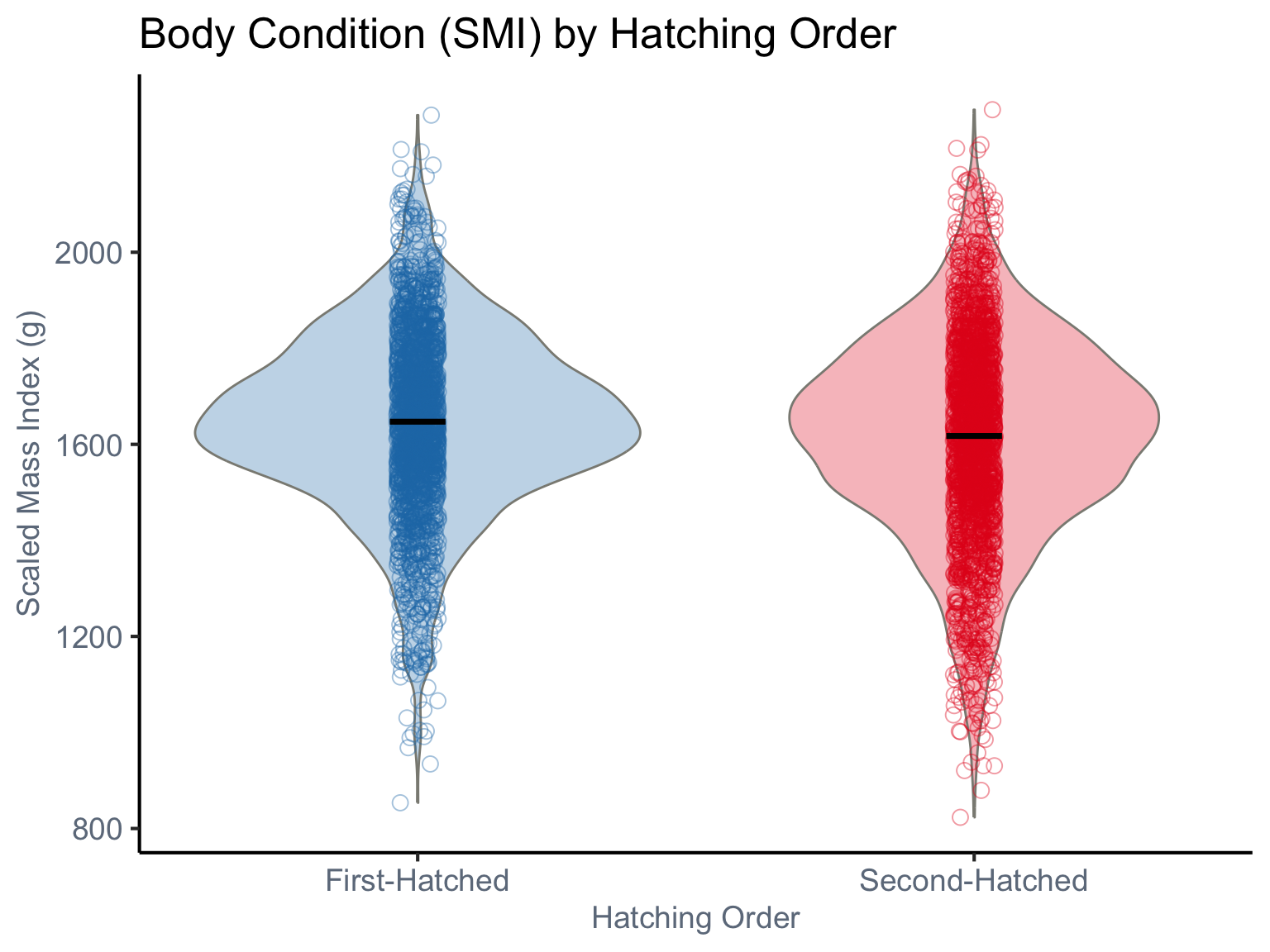
The plot displays the distribution of body condition, measured as Scaled Mass Index (SMI), for blue-footed booby chicks based on their hatching order. Violin plots illustrate the overall density distribution of SMI for both “First-Hatched” and “Second-Hatched” chicks. Each individual empty circle represents the SMI of a single chick. The plot visually highlights individual variability and allows for the comparison of both central tendency (black solid line) and spread of body condition between the two hatching orders.

dat <- read_csv(here("data","SMI_Drummond_et_al_2025.csv")) %>%subset(REDUCTION == 0)

dat<- dat%>%
  dplyr::select(-TIME, -HATCHING_DATE,-REDUCTION,-RING) %>%
  mutate(SMI = as.numeric(SMI),# Scaled mass index
         lnSMI=log(SMI),
         NEST = as.factor(NEST), 
         WORKYEAR = as.factor(WORKYEAR),
         RANK = factor(RANK, levels = c("1", "2")))


ggplot(dat, aes(x = RANK, y = SMI, fill = RANK, color = RANK)) +
 geom_violin(aes(fill = RANK),
              color = "#8B8B83",
              width = 0.8, 
              alpha = 0.3,
              position = position_dodge(width = 0.7)) +
  geom_jitter(aes(color = RANK),
              size = 3,
              alpha = 0.4,
              shape = 1,
              position = position_jitterdodge(dodge.width = 0.5, jitter.width = 0.15)) + 
  stat_summary(fun = mean,              
               geom = "crossbar",       
               width = 0.1,             
               color = "black",         
               linewidth = 0.5,         
               position = position_dodge(width = 0.7))+
  labs(
    title = "Body Condition (SMI) by Hatching Order",
    x = "Hatching Order",
    y = "Scaled Mass Index (g)"
  ) +
  scale_fill_manual(
    values = c("1" = "#1F78B4", "2" = "#E31A1C") # 
  ) +
  scale_color_manual(
    values = c("1" = "#1F78B4", "2" = "#E31A1C") # 
  ) +
  scale_x_discrete(
    labels = c("1" = "First-Hatched", "2" = "Second-Hatched"),
    expand = expansion(add = 0.5)
  ) +
  theme_classic(base_size = 16) +
  theme(
    axis.text = element_text(color = "#6E7B8B", size = 14),
    axis.title = element_text(color = "#6E7B8B", size = 14),
    legend.position = "none",
    axis.text.x = element_text(angle = 0, hjust = 0.5)
  )

3.3 Run models and interpret results

All models incorporate NEST_ID and YEAR random effects to account for non-independence of chicks within the same nest and observations within the same year.

The models are as follows:

Location-only model: Estimates the average difference in Scaled Mass Index (SMI) between the two hatching orders.
Location-scale model: Estimates both the average difference (location) and differences in the variability (scale) of SMI between hatching orders.

Following the previous section, we first fit a location-only model as our baseline and applied a log-transformation to SMI.

model2_1<-glmmTMB(lnSMI ~ 1 + RANK + (1|NEST)+(1|WORKYEAR),
              family = gaussian(), data=dat)

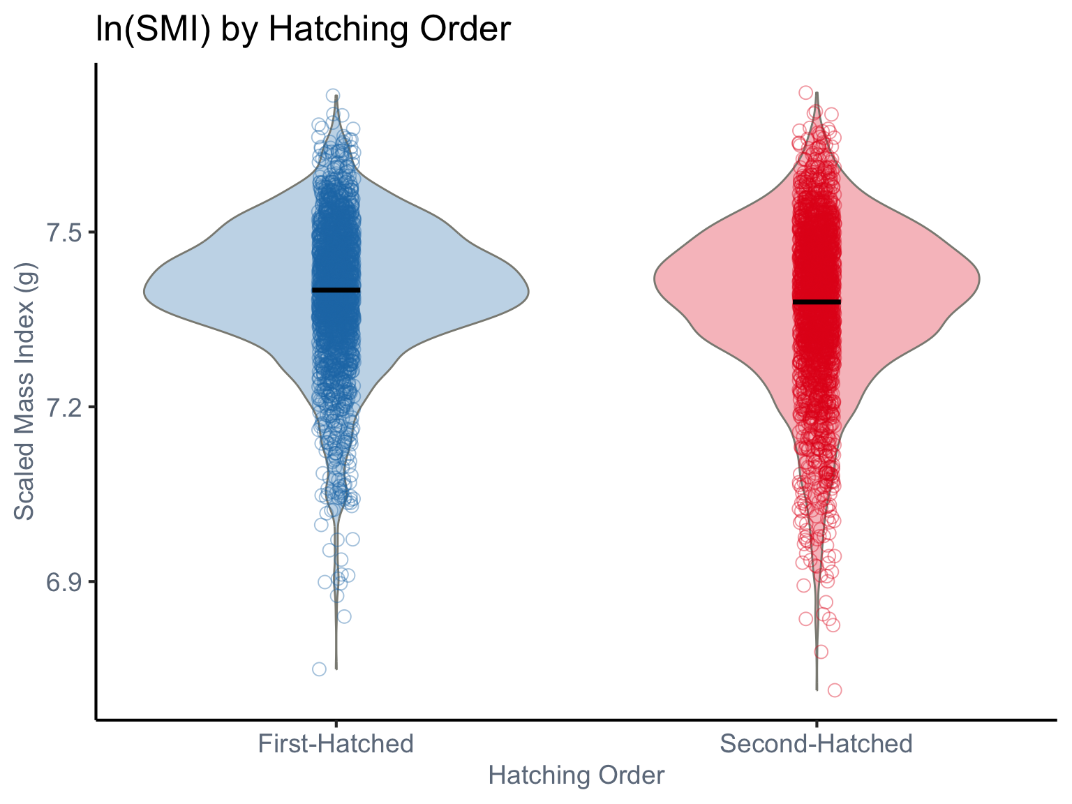
Rationale for Log-Transforming SMI Transforming the dependent variable to $log(SMI)$ is a standard approach used here for three primary reasons:

To Normalize Residuals: Mass data are typically right-skewed. The log transformation helps symmetrize the data’s distribution, making the model’s residuals better approximate the Gaussian distribution required by the family.

To Linearize Relationships: The log transform converts potentially non-linear, multiplicative relationships (common in biology) into the linear, additive relationships that are the foundation of this modeling framework.

To Address Heteroscedasticity: This transformation can help reduce heteroscedasticity, where variance increases with the mean. It’s a common first step to stabilize variance, though we will explicitly model the dispersion in subsequent models rather than relying solely on this transformation.

Code

ggplot(dat, aes(x = RANK, y = lnSMI, fill = RANK, color = RANK)) +
 geom_violin(aes(fill = RANK),
              color = "#8B8B83",
              width = 0.8, 
              alpha = 0.3,
              position = position_dodge(width = 0.7)) +
  geom_jitter(aes(color = RANK),
              size = 3,
              alpha = 0.4,
              shape = 1,
              position = position_jitterdodge(dodge.width = 0.5, jitter.width = 0.15)) + 
  stat_summary(fun = mean,              
               geom = "crossbar",       
               width = 0.1,             
               color = "black",         
               linewidth = 0.5,         
               position = position_dodge(width = 0.7))+
  labs(
    title = "ln(SMI) by Hatching Order",
    x = "Hatching Order",
    y = "Scaled Mass Index (g)"
  ) +
  scale_fill_manual(
    values = c("1" = "#1F78B4", "2" = "#E31A1C") # 
  ) +
  scale_color_manual(
    values = c("1" = "#1F78B4", "2" = "#E31A1C") # 
  ) +
  scale_x_discrete(
    labels = c("1" = "First-Hatched", "2" = "Second-Hatched"),
    expand = expansion(add = 0.5)
  ) +
  theme_classic(base_size = 16) +
  theme(
    axis.text = element_text(color = "#6E7B8B", size = 14),
    axis.title = element_text(color = "#6E7B8B", size = 14),
    legend.position = "none",
    axis.text.x = element_text(angle = 0, hjust = 0.5)
  )

summary(model2_1)

 Family: gaussian  ( identity )
Formula:          lnSMI ~ 1 + RANK + (1 | NEST) + (1 | WORKYEAR)
Data: dat

     AIC      BIC   logLik deviance df.resid 
 -8048.8  -8016.5   4029.4  -8058.8     4732 

Random effects:

Conditional model:
 Groups   Name        Variance Std.Dev.
 NEST     (Intercept) 0.002434 0.04934 
 WORKYEAR (Intercept) 0.008858 0.09412 
 Residual             0.008245 0.09080 
Number of obs: 4737, groups:  NEST, 2873; WORKYEAR, 24

Dispersion estimate for gaussian family (sigma^2): 0.00824 

Conditional model:
            Estimate Std. Error z value Pr(>|z|)    
(Intercept)  7.35953    0.01973   372.9  < 2e-16 ***
RANK2       -0.01872    0.00272    -6.9 5.91e-12 ***
---
Signif. codes:  0 '***' 0.001 '**' 0.01 '*' 0.05 '.' 0.1 ' ' 1

confint(model2_1)

                                   2.5 %      97.5 %    Estimate
(Intercept)                   7.32085592  7.39820911  7.35953252
RANK2                        -0.02405065 -0.01338785 -0.01871925
Std.Dev.(Intercept)|NEST      0.04463325  0.05454148  0.04933927
Std.Dev.(Intercept)|WORKYEAR  0.07008890  0.12638674  0.09411859

Interpreting Log-Level Model Coefficients

Since the outcome is logged, this is a log-level model. A coefficient for a categorical predictor like RANK represents a multiplicative change on the original SMI scale.

To interpret a coefficient ($\beta$) for a given level of RANK relative to the reference level, you must exponentiate it.

Multiplicative Factor on SMI: \[ \text{Factor} = e^{\beta} \]
Percentage Change in SMI: \[ \text{Change} = (e^{\beta} - 1) \times 100\% \]

3.3.0.1 Example:

Our model estimates the coefficient for RANK = ‘junior’ to be -0.018 (with ‘senior’ as the reference level):

Calculate the multiplicative factor: \[ e^{-0.018} \approx 0.982 \]
Convert to a percentage change: \[ (0.982 - 1) \times 100\% = -1.7\% \]

The concise interpretation is:

“The scaled mass index for second-hatched individuals is, on average, 1.7% lower than that of the first-hatched reference group.”

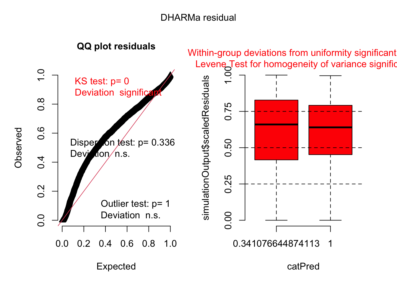
Then we use the ‘DHARMa’ package to simulate residuals and plot them automatically. This step is crucial for checking the model’s assumptions, such as normality and homoscedasticity of residuals.

# | label: model_diagnostics - model0
simulationOutput <- simulateResiduals(fittedModel = model2_1, plot = F)
plot(simulationOutput)

The QQ plot and Kolmogorov-Smirnov (KS) test reveal that the model’s residuals aren’t uniformly distributed, hinting at potential issues with the chosen distribution or the model’s underlying structure. While tests for overdispersion and outliers showed no significant concerns, the boxplots and Levene test highlight a lack of uniformity within residual groups and non-homogeneous variances. This suggests the model doesn’t fully capture the data’s complexity and might benefit from adjustments, perhaps by incorporating a location-scale model to better handle varying dispersion.

# location-scale model ---- 

model2_2 <- glmmTMB(
    lnSMI ~ 1 + RANK + (1|NEST)+(1|WORKYEAR),
    dispformula = ~ 1 + RANK,     
    data = dat, 
    family = gaussian
    )
summary(model2_2)

 Family: gaussian  ( identity )
Formula:          lnSMI ~ 1 + RANK + (1 | NEST) + (1 | WORKYEAR)
Dispersion:             ~1 + RANK
Data: dat

     AIC      BIC   logLik deviance df.resid 
 -8070.8  -8032.1   4041.4  -8082.8     4731 

Random effects:

Conditional model:
 Groups   Name        Variance Std.Dev.
 NEST     (Intercept) 0.002430 0.04929 
 WORKYEAR (Intercept) 0.008595 0.09271 
 Residual                   NA      NA 
Number of obs: 4737, groups:  NEST, 2873; WORKYEAR, 24

Conditional model:
            Estimate Std. Error z value Pr(>|z|)    
(Intercept)  7.36075    0.01944   378.7  < 2e-16 ***
RANK2       -0.01880    0.00271    -6.9 3.93e-12 ***
---
Signif. codes:  0 '***' 0.001 '**' 0.01 '*' 0.05 '.' 0.1 ' ' 1

Dispersion model:
            Estimate Std. Error z value Pr(>|z|)    
(Intercept) -2.47026    0.02242 -110.20  < 2e-16 ***
RANK2        0.13035    0.02687    4.85 1.23e-06 ***
---
Signif. codes:  0 '***' 0.001 '**' 0.01 '*' 0.05 '.' 0.1 ' ' 1

confint(model2_2)

                                        2.5 %      97.5 %    Estimate
cond.(Intercept)                   7.32265786  7.39885037  7.36075412
cond.RANK2                        -0.02411510 -0.01349325 -0.01880417
disp.(Intercept)                  -2.51419214 -2.42631943 -2.47025578
disp.RANK2                         0.07768165  0.18301526  0.13034846
cond.Std.Dev.(Intercept)|NEST      0.04462552  0.05445269  0.04929482
cond.Std.Dev.(Intercept)|WORKYEAR  0.06903183  0.12450065  0.09270657

Interpreting Location-Scale Model Coefficients

Location Model: Mean (Conditional model)
Scale Model: Variability (Dispersion model)

This component predicts the mean of $log(SMI)$. Because it’s on the log scale, coefficients translate into percentage changes in SMI.

RANK2 Coefficient = -0.01880

Multiplicative factor: $e^{-0.01880} \approx 0.981$

Percentage change: $-1.86%$

Interpretation: Individuals in RANK2 have, on average, a 1.9% lower SMI than those in RANK1.

This component models the residual standard deviation ($σ$) of log(SMI). Since $σ$ is constrained to be positive, the model uses a log link, so coefficients are exponentiated and interpreted as percentage changes in variability.

RANK2 Coefficient = 0.13035

Multiplicative factor: $e^{0.13035} \approx 1.14$

Percentage change: $+14.0%$

Interpretation: The residual variability in log(SMI) for RANK2 individuals is 14% higher than for RANK1, meaning their SMI values are more variable.

Finally, we compare the location-scale model with the location-only model based on AICc values (model.sel() from the MuMIn package).

model.sel(model2_1, model2_2)

The results of the location-only model (Model 0) and the location-scale model (Model 1) are summarized below.

Location-only model
Term	Estimate	Std. Error	95% CI (low)	95% CI (high)
(Intercept)	7.360	0.020	7.321	7.398
RANK2	−0.019	0.003	−0.024	−0.013

Location-scale model (location part)
Term	Estimate	Std. Error	95% CI (low)	95% CI (high)
(Intercept)	7.361	0.019	7.323	7.399
RANK2	−0.019	0.003	−0.024	−0.013

Location-scale model (dispersion part)
Term	Estimate	Std. Error	95% CI (low)	95% CI (high)
(Intercept)	−2.470	0.022	−2.514	−2.426
RANK2	0.130	0.027	0.078	0.183

emm_location <- emmeans(model2_2, ~ RANK,
                        component = "cond", type = "link")
df_location <- as.data.frame(emm_location) %>%
  rename(
    mean_log = emmean, 
    lwr = lower.CL,    
    upr = upper.CL     
  )
emm_dispersion <- emmeans(model2_2, ~ RANK,
                          component = "disp", type = "response")
df_dispersion <- as.data.frame(emm_dispersion) %>%
  rename(
    log_sigma = response, 
    lwr = lower.CL,     
    upr = upper.CL     
  )
pos <- position_dodge(width = 0.4)


plot_location_emmeans <- ggplot(df_location, aes(x = RANK, y = mean_log)) +
  geom_point(position = pos, size = 3) +
  geom_errorbar(aes(ymin = lwr, ymax = upr), position = pos, width = 0.15) +
  labs(
    title = "Location",
    x = "Hatching order",
    y = "log(SMI)"
  ) +
  theme_classic()+ scale_y_continuous(breaks = seq(7.2,7.5,0.05),limits = c(7.2, 7.5))

plot_dispersion_emmeans <- ggplot(df_dispersion, aes(x = RANK, y = log_sigma)) +
  geom_point(position = pos, size = 3) +
  geom_errorbar(aes(ymin = lwr, ymax = upr), position = pos, width = 0.15) +
  labs(
    title = "Scale",
    x = "Hatching order",
    y = "Standard Deviation"
  ) +
  theme_classic() + scale_y_continuous(breaks = seq(0.07,0.12,0.01),limits = c(0.07, 0.12))

plot_location_emmeans + plot_dispersion_emmeans

3.4 Bonus

Here is how to fit the same location-scale models using the brms package for comparison.

m1 <- bf(log(SMI) ~ 1 + RANK + (1|NEST) + (1|WORKYEAR))
prior1<-default_prior(m1, data = dat, family = gaussian())

fit1 <- brm(
  m1,
  prior = prior1,
  data = dat,
  family = gaussian(),
  iter = 6000,     
  warmup = 1000,   
  chains = 4,  cores=4,
  backend = "cmdstanr",
  control = list(
    adapt_delta = 0.99,  # Keep high if you have divergent transitions
    max_treedepth = 15   # Keep high if hitting max_treedepth warnings
    ),
  seed = 123,      
  refresh = 500    # Less frequent progress updates (reduces overhead)
)

 Family: gaussian 
  Links: mu = identity 
Formula: log(SMI) ~ (1 | NEST) + (1 | WORKYEAR) + RANK 
   Data: dat (Number of observations: 4737) 
  Draws: 4 chains, each with iter = 6000; warmup = 1000; thin = 1;
         total post-warmup draws = 20000

Multilevel Hyperparameters:
~NEST (Number of levels: 2873) 
              Estimate Est.Error l-95% CI u-95% CI Rhat Bulk_ESS Tail_ESS
sd(Intercept)     0.05      0.00     0.04     0.05 1.00     4028     7765

~WORKYEAR (Number of levels: 24) 
              Estimate Est.Error l-95% CI u-95% CI Rhat Bulk_ESS Tail_ESS
sd(Intercept)     0.10      0.02     0.08     0.14 1.00     5145     9062

Regression Coefficients:
          Estimate Est.Error l-95% CI u-95% CI Rhat Bulk_ESS Tail_ESS
Intercept     7.36      0.02     7.32     7.40 1.00     2947     5200
RANK2        -0.02      0.00    -0.02    -0.01 1.00    25883    12974

Further Distributional Parameters:
      Estimate Est.Error l-95% CI u-95% CI Rhat Bulk_ESS Tail_ESS
sigma     0.09      0.00     0.09     0.09 1.00     5732    10919

Draws were sampled using sample(hmc). For each parameter, Bulk_ESS
and Tail_ESS are effective sample size measures, and Rhat is the potential
scale reduction factor on split chains (at convergence, Rhat = 1).

m2 <- bf(log(SMI) ~ 1 + RANK + (1|NEST) + (1|WORKYEAR),
         sigma~ 1 + RANK)
prior2 <- default_prior(m2,data = dat,family = gaussian())

fit2 <- brm(
 m2,
 prior= prior2,
 data = dat,
 family = gaussian(),
 iter = 6000,     
 warmup = 1000,   
 chains = 4,  cores=4,
 backend = "cmdstanr",
 control = list(
   adapt_delta = 0.99,  # Keep high if you have divergent transitions
   max_treedepth = 15   # Keep high if hitting max_treedepth warnings
 ),
 seed = 123,      
 refresh = 500    # Less frequent progress updates (reduces overhead)
)

 Family: gaussian 
  Links: mu = identity; sigma = log 
Formula: log(SMI) ~ 1 + RANK + (1 | NEST) + (1 | WORKYEAR) 
         sigma ~ 1 + RANK
   Data: dat (Number of observations: 4737) 
  Draws: 4 chains, each with iter = 6000; warmup = 1000; thin = 1;
         total post-warmup draws = 20000

Multilevel Hyperparameters:
~NEST (Number of levels: 2873) 
              Estimate Est.Error l-95% CI u-95% CI Rhat Bulk_ESS Tail_ESS
sd(Intercept)     0.05      0.00     0.04     0.05 1.00     3871     8155

~WORKYEAR (Number of levels: 24) 
              Estimate Est.Error l-95% CI u-95% CI Rhat Bulk_ESS Tail_ESS
sd(Intercept)     0.10      0.02     0.07     0.14 1.00     3937     7503

Regression Coefficients:
                Estimate Est.Error l-95% CI u-95% CI Rhat Bulk_ESS Tail_ESS
Intercept           7.36      0.02     7.32     7.40 1.00     1826     4007
sigma_Intercept    -2.47      0.02    -2.51    -2.43 1.00     5963    11191
RANK2              -0.02      0.00    -0.02    -0.01 1.00    31665    14172
sigma_RANK2         0.13      0.03     0.08     0.18 1.00    16024    15761

Draws were sampled using sample(hmc). For each parameter, Bulk_ESS
and Tail_ESS are effective sample size measures, and Rhat is the potential
scale reduction factor on split chains (at convergence, Rhat = 1).

f1loo <- loo::loo(fit1)
f2loo <- loo::loo(fit2)

#Model comparison 
fc <- loo::loo_compare(f1loo, f2loo)
fc

#     elpd_diff se_diff
# fit2   0.0       0.0  
# fit1 -10.3       7.6

LOO (Leave-One-Out) model comparison helps us estimate which Bayesian model will best predict new data. The elpd_diff (Estimated Log Predictive Density difference) tells us the difference in predictive accuracy, with a more positive number indicating better performance. The se_diff (Standard Error of the Difference) provides the uncertainty around this difference. In our results, fit2 (the location-scale model) has an elpd_diff of 0.0, meaning it’s the reference or best-performing model. fit1 (the location-only model) has an elpd_diff of -10.3 with an se_diff of 7.6, indicating that fit2 is estimated to be substantially better at predicting new data than fit1, although there is some uncertainty in that difference. As a rule of thumb, if the absolute value of the elpd_diff is more than twice the se_diff, we can consider the difference as meaningful ($|elpd\_diff| > 2 * se\_diff$).

Model 1: Posterior Summary
Term	Estimate	Std.error	95% CI (low)	95% CI (high)
Location Model
Intercept	7.359	0.022	7.316	7.403
Second hatched chick	−0.019	0.003	−0.024	−0.013
Random Effects
Nest ID	0.049	0.003	0.044	0.054
Year	0.102	0.017	0.075	0.141
Residual Standard Deviation
Sigma	0.091	0.001	0.088	0.094

Model 2: Posterior Summary
Term	Estimate	Std.error	95% CI (low)	95% CI (high)
Location Submodel
Intercept	7.360	0.021	7.318	7.402
Second hatched chick	−0.019	0.003	−0.024	−0.014
Scale Submodel
Intercept (sigma)	−2.469	0.022	−2.514	−2.426
Second hatched chick (sigma)	0.130	0.027	0.077	0.182
Random effects
Nest ID	0.049	0.003	0.044	0.054
Year	0.100	0.017	0.073	0.139

The location-scale model (Model 2) was the most-supported model based on AICc values (-8070.8) compared to the location-only model (-8048.8; see Model comparison tab for details).

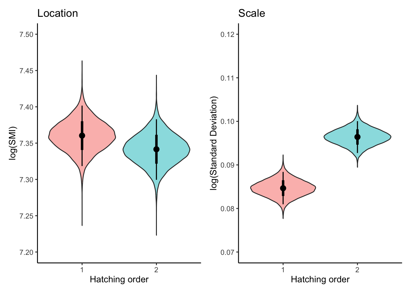
m2_draws<-fit2 %>%
  tidybayes::epred_draws(newdata = expand.grid(
    RANK = unique(dat$RANK)
  ), re_formula = NA, dpar =TRUE) 


plot_lm2 <- ggplot(m2_draws, aes(x = factor(RANK), y = .epred,fill = factor(RANK))) +
  geom_violin(alpha = 0.5, show.legend = FALSE)+
  stat_pointinterval(show.legend = FALSE) +
  labs(
    title = "Location",
    x = "Hatching order", 
    y = "log(SMI)"
  ) +
  theme_classic() + scale_y_continuous(breaks = seq(7.2,7.5,0.05),limits = c(7.2, 7.5))


plot_sm2 <- ggplot(m2_draws, aes(x = factor(RANK), y = sigma,fill = factor(RANK))) +
geom_violin(alpha = 0.5, show.legend = FALSE)+
  stat_pointinterval(show.legend = FALSE) +
  labs(
    title = "Scale",
    x = "Hatching order", 
    y = "log(Standard Deviation)"
  ) +
  theme_classic() + scale_y_continuous(breaks = seq(0.07,0.12,0.01),limits = c(0.07, 0.12))

combinded_plot<-(plot_lm2 + plot_sm2)& 
  theme(
    panel.grid.major = element_blank(), 
    panel.grid.minor = element_blank()
  )
combinded_plot

The Challenge: Summarized Data vs. Distributional Plots

A violin plot is a powerful tool for visualizing the entire distribution of a dataset. To draw its characteristic shape, ggplot2::geom_violin() needs the full “cloud” of possible values to calculate the data’s density at different points.

However, many traditional analysis functions are designed to provide summarized marginal means, not raw posterior draws. For example, when you use a function like emmeans() on a frequentist model, it calculates a single point estimate (like a mean) and a confidence interval for each group.

The resulting data frame is already summarized. This summary data lacks the thousands of individual data points needed to describe a distribution’s shape. geom_violin() simply cannot work with this, as it has no information about the density of the predictions, only their central tendency and range.

The brms Solution: The Full Posterior Distribution

This is where the Bayesian workflow with brms and tidybayes excels. The tidybayes::epred_draws() function is specifically designed to extract the full posterior distribution from your brms model and provide it as a tidy, long-format data frame.

Instead of a single summary row per group, epred_draws() gives you thousands of rows—one for each posterior draw from your model. This data frame represents the entire “cloud” of possible values that geom_violin() needs.

By providing the complete posterior distribution in a clean, plot-ready format, the brms and tidybayes ecosystem makes creating rich, distributional visualizations like violin plots a natural and direct step in the analysis workflow.

Point estimates
Posterior distribution

#| echo: false


plot_location_emmeans + plot_dispersion_emmeans

3.5 Interpretation of location-scale model :

Location (mean) part:

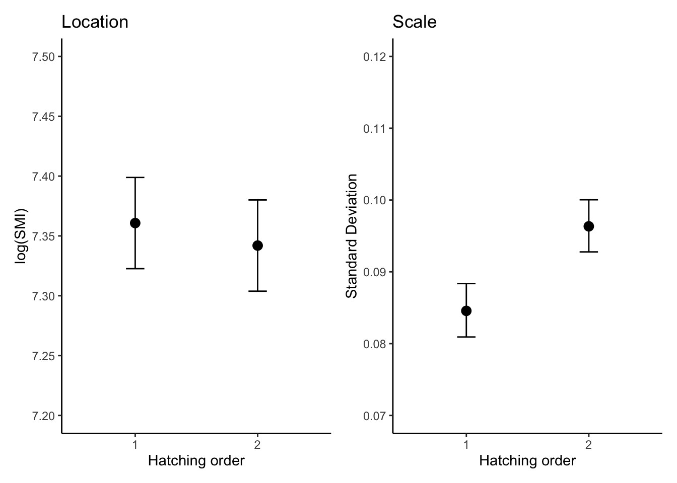
There was a conclusive effect of hatching order on the mean of log(SMI), with second-hatched chicks having a lower SMI than first-hatched chicks ($\beta_{[\text{first-second}]}^{(l)}$ = -0.018, 95% CI = [-0.024, -0.013]).In percentage terms, the SMI for second-hatched chicks is estimated to be 1.8% lower than for first-hatched chicks

Scale (dispersion) part:

The scale component revealed a conclusive difference in the variability of SMI between hatching orders. The second-hatched chicks exhibited greater variability in SMI compared to first-hatched chicks ($\beta_{[\text{first-second}]}^{(s)}$ = 0.130, 95% CI = [0.077, 0.183]).This means the standard deviation of SMI for second-hatched chicks is 13.9% higher than for first-hatched chicks

Location (mean) random effects:

There is very little variation in the average body condition across different nests ($\sigma_{[\text{Nest\_ID}]}^{(l)}$ = 0.049, 95% CI [0.044, 0.054]), suggesting that most nests have similar average body conditions for their chicks.
There is also very little variation in the average body condition across different years ($\sigma_{[\text{Year}]}^{(l)}$ = 0.092, 95% CI [0.069, 0.124]),implying generally consistent average body conditions from year to year.

3.6 Conclusion

Do first hatched chicks have a higher body mass than second-hatched chicks?

Answer: Answer: Yes, first-hatched chicks have a significantly higher Scaled Mass Index (SMI) than second-hatched chicks at fledgling, with a mean difference of approximately 0.018 on the log scale.

Does the variability in body mass differ between first and second-hatched chicks?

Answer: Yes, the variability in body mass (SMI) is significantly greater in second-hatched chicks compared to first-hatched chicks. This indicates that second-hatched chicks show more variation in their body condition at fledgling.

--- title: "Adding random effects in the location part only (model 2)" --- ```{r} #| label: load_packages #| echo: false # Load required packages pacman::p_load( ## data manipulation dplyr, tibble, tidyverse, broom, broom.mixed, ## model fitting ape, arm, brms, broom.mixed, cmdstanr, emmeans, ggeffects, glmmTMB, MASS, phytools, rstan, TreeTools, ## model checking and evaluation DHARMa, loo, MuMIn, parallel, ## visualisation bayesplot, ggplot2, patchwork, tidybayes, ## reporting and utilities gt, here, kableExtra, knitr ) ``` Model 2 is a location-scale model with random effects in the location part only. This allows us to account for individual-level variation in the mean response while still modeling the dispersion separately. ## Dataset overview This dataset comes from [Drummond et al (2025)](https://doi.org/10.1093/beheco/araf050), which examined the benefits of brood reduction in the blue-footed booby (*Sula nebouxii*).Focusing on two-chick broods, the research explored whether the death of one chick (brood reduction) primarily benefits the surviving sibling (via increased resource acquisition) or the parents (by lessening parental investment). In this species, older chicks establish a strong dominance hierarchy over their younger siblings. Under stressful environmental conditions, this often results in the death of the second-hatched chick, with parental intervention being extremely rare. For this tutorial, we will specifically examine data from two-chick broods where both chicks survived to fledgling. Our analysis will focus on how hatching order influences the body condition of chicks at fledgling. ### Questions 1. **Do first hatched chicks have a higher body mass than second-hatched chicks?** 2. **Does the variability in body mass differ between first and second-hatched chicks?** ### Variables included ::: {.callout-note appearance="simple" icon="false"} - `SMI`: Scaled Mass Index, a measure that accounts for body mass relative to size - `RANK`: The order in which chicks hatched (1 for first-hatched, 2 for second-hatched) - `NEST_ID`: Identifier for the nest where the chicks were raised - `YEAR`: The year in which the chicks were born ::: ## Visualise the dataset The plot displays the distribution of body condition, measured as Scaled Mass Index (SMI), for blue-footed booby chicks based on their `hatching order`. Violin plots illustrate the overall density distribution of SMI for both "First-Hatched" and "Second-Hatched" chicks. Each individual empty circle represents the SMI of a single chick. The plot visually highlights individual variability and allows for the comparison of both central tendency (black solid line) and spread of body condition between the two hatching orders. ```{r} #| label: show_data - model2 #| fig-width: 8 #| fig-height: 6 dat <- read_csv(here("data","SMI_Drummond_et_al_2025.csv")) %>%subset(REDUCTION == 0) dat<- dat%>% dplyr::select(-TIME, -HATCHING_DATE,-REDUCTION,-RING) %>% mutate(SMI = as.numeric(SMI),# Scaled mass index lnSMI=log(SMI), NEST = as.factor(NEST), WORKYEAR = as.factor(WORKYEAR), RANK = factor(RANK, levels = c("1", "2"))) ggplot(dat, aes(x = RANK, y = SMI, fill = RANK, color = RANK)) + geom_violin(aes(fill = RANK), color = "#8B8B83", width = 0.8, alpha = 0.3, position = position_dodge(width = 0.7)) + geom_jitter(aes(color = RANK), size = 3, alpha = 0.4, shape = 1, position = position_jitterdodge(dodge.width = 0.5, jitter.width = 0.15)) + stat_summary(fun = mean, geom = "crossbar", width = 0.1, color = "black", linewidth = 0.5, position = position_dodge(width = 0.7))+ labs( title = "Body Condition (SMI) by Hatching Order", x = "Hatching Order", y = "Scaled Mass Index (g)" ) + scale_fill_manual( values = c("1" = "#1F78B4", "2" = "#E31A1C") # ) + scale_color_manual( values = c("1" = "#1F78B4", "2" = "#E31A1C") # ) + scale_x_discrete( labels = c("1" = "First-Hatched", "2" = "Second-Hatched"), expand = expansion(add = 0.5) ) + theme_classic(base_size = 16) + theme( axis.text = element_text(color = "#6E7B8B", size = 14), axis.title = element_text(color = "#6E7B8B", size = 14), legend.position = "none", axis.text.x = element_text(angle = 0, hjust = 0.5) ) ``` ## Run models and interpret results All models incorporate `NEST_ID` and `YEAR` random effects to account for non-independence of chicks within the same nest and observations within the same year. The models are as follows: a. Location-only model: Estimates the average difference in Scaled Mass Index (SMI) between the two hatching orders. b. Location-scale model: Estimates both the average difference (location) and differences in the variability (scale) of SMI between hatching orders. ::: panel-tabset ## Location model Following the previous section, we first fit a location-only model as our baseline and applied a log-transformation to `SMI`. ```{r} #| label: model_fitting2-model1 model2_1<-glmmTMB(lnSMI ~ 1 + RANK + (1|NEST)+(1|WORKYEAR), family = gaussian(), data=dat) ``` ::: {.callout-note appearance="simple" icon="false"} Rationale for Log-Transforming SMI Transforming the dependent variable to $log(SMI)$ is a standard approach used here for three primary reasons: To Normalize Residuals: Mass data are typically right-skewed. The log transformation helps symmetrize the data's distribution, making the model's residuals better approximate the Gaussian distribution required by the family. To Linearize Relationships: The log transform converts potentially non-linear, multiplicative relationships (common in biology) into the linear, additive relationships that are the foundation of this modeling framework. To Address Heteroscedasticity: This transformation can help reduce heteroscedasticity, where variance increases with the mean. It's a common first step to stabilize variance, though we will explicitly model the dispersion in subsequent models rather than relying solely on this transformation. ```{r} #| label: show_data - model2_log #| fig-width: 8 #| fig-height: 6 #| code-fold: true ggplot(dat, aes(x = RANK, y = lnSMI, fill = RANK, color = RANK)) + geom_violin(aes(fill = RANK), color = "#8B8B83", width = 0.8, alpha = 0.3, position = position_dodge(width = 0.7)) + geom_jitter(aes(color = RANK), size = 3, alpha = 0.4, shape = 1, position = position_jitterdodge(dodge.width = 0.5, jitter.width = 0.15)) + stat_summary(fun = mean, geom = "crossbar", width = 0.1, color = "black", linewidth = 0.5, position = position_dodge(width = 0.7))+ labs( title = "ln(SMI) by Hatching Order", x = "Hatching Order", y = "Scaled Mass Index (g)" ) + scale_fill_manual( values = c("1" = "#1F78B4", "2" = "#E31A1C") # ) + scale_color_manual( values = c("1" = "#1F78B4", "2" = "#E31A1C") # ) + scale_x_discrete( labels = c("1" = "First-Hatched", "2" = "Second-Hatched"), expand = expansion(add = 0.5) ) + theme_classic(base_size = 16) + theme( axis.text = element_text(color = "#6E7B8B", size = 14), axis.title = element_text(color = "#6E7B8B", size = 14), legend.position = "none", axis.text.x = element_text(angle = 0, hjust = 0.5) ) ``` ::: ```{r} summary(model2_1) confint(model2_1) ``` ::: {.callout-note appearance="simple" icon="false"} ### Interpreting Log-Level Model Coefficients Since the outcome is logged, this is a log-level model. A coefficient for a categorical predictor like `RANK` represents a multiplicative change on the original `SMI` scale. To interpret a coefficient ($\beta$) for a given level of `RANK` relative to the reference level, you must exponentiate it. * **Multiplicative Factor on SMI:** $$ \text{Factor} = e^{\beta} $$ * **Percentage Change in SMI:** $$ \text{Change} = (e^{\beta} - 1) \times 100\% $$ #### Example: Our model estimates the coefficient for `RANK` = 'junior' to be **-0.018** (with 'senior' as the reference level): 1. **Calculate the multiplicative factor:** $$ e^{-0.018} \approx 0.982 $$ 2. **Convert to a percentage change:** $$ (0.982 - 1) \times 100\% = -1.7\% $$ The concise interpretation is: "The scaled mass index for second-hatched individuals is, on average, **1.7% lower** than that of the first-hatched reference group." ::: ## Model diagnostics Then we use the 'DHARMa' package to simulate residuals and plot them automatically. This step is crucial for checking the model's assumptions, such as normality and homoscedasticity of residuals. ```{r} # | label: model_diagnostics - model0 simulationOutput <- simulateResiduals(fittedModel = model2_1, plot = F) plot(simulationOutput) ``` The QQ plot and Kolmogorov-Smirnov (KS) test reveal that the model's residuals aren't uniformly distributed, hinting at potential issues with the chosen distribution or the model's underlying structure. While tests for overdispersion and outliers showed no significant concerns, the boxplots and Levene test highlight a lack of uniformity within residual groups and non-homogeneous variances. This suggests the model doesn't fully capture the data's complexity and might benefit from adjustments, perhaps by incorporating a location-scale model to better handle varying dispersion. ## Location-scale model ```{r} #| label: model_fitting2 - model2 - glmmtmb # location-scale model ---- model2_2 <- glmmTMB( lnSMI ~ 1 + RANK + (1|NEST)+(1|WORKYEAR), dispformula = ~ 1 + RANK, data = dat, family = gaussian ) summary(model2_2) confint(model2_2) ``` ::: {.callout-note appearance="simple" icon="false"} Interpreting Location-Scale Model Coefficients ::: panel-tabset ## Location Model: Mean (Conditional model) This component predicts the mean of $log(SMI)$. Because it’s on the log scale, coefficients translate into percentage changes in SMI. RANK2 Coefficient = -0.01880 Multiplicative factor: $e^{-0.01880} \approx 0.981$ Percentage change: $-1.86%$ Interpretation: Individuals in RANK2 have, on average, a 1.9% lower SMI than those in RANK1. ## Scale Model: Variability (Dispersion model) This component models the residual standard deviation ($σ$) of log(SMI). Since $σ$ is constrained to be positive, the model uses a log link, so coefficients are exponentiated and interpreted as percentage changes in variability. RANK2 Coefficient = 0.13035 Multiplicative factor: $e^{0.13035} \approx 1.14$ Percentage change: $+14.0%$ Interpretation: The residual variability in log(SMI) for RANK2 individuals is 14% higher than for RANK1, meaning their SMI values are more variable. ::: ::: ## Model comparison Finally, we compare the location-scale model with the location-only model based on AICc values (`model.sel()` from the `MuMIn` package). ```{r} #| label: model_comparison - model2 - glmmtmb model.sel(model2_1, model2_2) ``` ## Summary of model results The results of the location-only model (Model 0) and the location-scale model (Model 1) are summarized below. ```{r} #| echo: false #| label: model2_1_results - glmmtmb coefs_0 <- summary(model2_1)$coefficients$cond conf_0 <- confint(model2_1) rownames(conf_0) <- gsub("^cond\\.", "", rownames(conf_0)) conf_0 <- conf_0[rownames(conf_0) %in% rownames(coefs_0), ] match_0 <- match(rownames(coefs_0), rownames(conf_0)) results_0 <- data.frame( Term = rownames(coefs_0), Estimate = coefs_0[, "Estimate"], StdError = coefs_0[, "Std. Error"], `2.5%` = conf_0[match_0, "2.5 %"], `97.5%` = conf_0[match_0, "97.5 %"] ) colnames(results_0)[which(names(results_0) == "X2.5.")] <- "CI_low" colnames(results_0)[which(names(results_0) == "X97.5.")] <- "CI_high" gt(results_0) %>% tab_header(title = "Location-only model") %>% fmt_number(columns = everything(), decimals = 3) %>% cols_label( Term = "Term", Estimate = "Estimate", StdError = "Std. Error", CI_low = "95% CI (low)", CI_high = "95% CI (high)" ) %>% cols_align(align = "center", columns = everything()) ``` ```{r} #| echo: false #| label: model2_2_results - glmmtmb # Location-scale model (Model 1) ---- summary_1 <- summary(model2_2) conf_1 <- confint(model2_2) ## location part ---- coefs_1_loc <- summary_1$coefficients$cond conf_1_loc <- conf_1[grep("^cond", rownames(conf_1)), ] rownames(conf_1_loc) <- gsub("^cond\\.", "", rownames(conf_1_loc)) conf_1_loc <- conf_1_loc[rownames(conf_1_loc) %in% rownames(coefs_1_loc), ] match_loc <- match(rownames(coefs_1_loc), rownames(conf_1_loc)) results_1_loc <- data.frame( Term = rownames(coefs_1_loc), Estimate = coefs_1_loc[, "Estimate"], StdError = coefs_1_loc[, "Std. Error"], CI_low = conf_1_loc[match_loc, "2.5 %"], CI_high = conf_1_loc[match_loc, "97.5 %"] ) colnames(results_1_loc)[which(names(results_1_loc) == "X2.5.")] <- "CI_low" colnames(results_1_loc)[which(names(results_1_loc) == "X97.5.")] <- "CI_high" ## dispersion part ---- coefs_1_disp <- summary_1$coefficients$disp conf_1_disp <- conf_1[grep("^disp", rownames(conf_1)), ] rownames(conf_1_disp) <- gsub("^disp\\.", "", rownames(conf_1_disp)) conf_1_disp <- conf_1_disp[rownames(conf_1_disp) %in% rownames(coefs_1_disp), ] match_disp <- match(rownames(coefs_1_disp), rownames(conf_1_disp)) results_1_disp <- data.frame( Term = rownames(coefs_1_disp), Estimate = coefs_1_disp[, "Estimate"], StdError = coefs_1_disp[, "Std. Error"], CI_low = conf_1_disp[match_disp, "2.5 %"], CI_high = conf_1_disp[match_disp, "97.5 %"] ) colnames(results_1_loc)[which(names(results_1_disp) == "X2.5.")] <- "CI_low" colnames(results_1_loc)[which(names(results_1_disp) == "X97.5.")] <- "CI_high" # display results ---- gt(results_1_loc) %>% tab_header(title = "Location-scale model (location part)") %>% fmt_number(columns = everything(), decimals = 3) %>% cols_label( Term = "Term", Estimate = "Estimate", StdError = "Std. Error", CI_low = "95% CI (low)", CI_high = "95% CI (high)" ) %>% cols_align(align = "center", columns = everything()) gt(results_1_disp) %>% tab_header(title = "Location-scale model (dispersion part)") %>% fmt_number(columns = everything(), decimals = 3) %>% cols_label( Term = "Term", Estimate = "Estimate", StdError = "Std. Error", CI_low = "95% CI (low)", CI_high = "95% CI (high)" ) %>% cols_align(align = "center", columns = everything()) ``` ## Figures ```{r} #| label: emmeans_plots - model2 - glmmtmb emm_location <- emmeans(model2_2, ~ RANK, component = "cond", type = "link") df_location <- as.data.frame(emm_location) %>% rename( mean_log = emmean, lwr = lower.CL, upr = upper.CL ) emm_dispersion <- emmeans(model2_2, ~ RANK, component = "disp", type = "response") df_dispersion <- as.data.frame(emm_dispersion) %>% rename( log_sigma = response, lwr = lower.CL, upr = upper.CL ) pos <- position_dodge(width = 0.4) plot_location_emmeans <- ggplot(df_location, aes(x = RANK, y = mean_log)) + geom_point(position = pos, size = 3) + geom_errorbar(aes(ymin = lwr, ymax = upr), position = pos, width = 0.15) + labs( title = "Location", x = "Hatching order", y = "log(SMI)" ) + theme_classic()+ scale_y_continuous(breaks = seq(7.2,7.5,0.05),limits = c(7.2, 7.5)) plot_dispersion_emmeans <- ggplot(df_dispersion, aes(x = RANK, y = log_sigma)) + geom_point(position = pos, size = 3) + geom_errorbar(aes(ymin = lwr, ymax = upr), position = pos, width = 0.15) + labs( title = "Scale", x = "Hatching order", y = "Standard Deviation" ) + theme_classic() + scale_y_continuous(breaks = seq(0.07,0.12,0.01),limits = c(0.07, 0.12)) plot_location_emmeans + plot_dispersion_emmeans ``` ::: ## Bonus Here is how to fit the same location-scale models using the `brms` package for comparison. ::: panel-tabset ## Location-only model  ```{r} #| label: model_fitting1 - model2 - brms #| eval: false m1 <- bf(log(SMI) ~ 1 + RANK + (1|NEST) + (1|WORKYEAR)) prior1<-default_prior(m1, data = dat, family = gaussian()) fit1 <- brm( m1, prior = prior1, data = dat, family = gaussian(), iter = 6000, warmup = 1000, chains = 4, cores=4, backend = "cmdstanr", control = list( adapt_delta = 0.99, # Keep high if you have divergent transitions max_treedepth = 15 # Keep high if hitting max_treedepth warnings ), seed = 123, refresh = 500 # Less frequent progress updates (reduces overhead) ) ``` ```{r} #| label: model1_result - model2 - brms #| echo: false fit1 <- readRDS(here("Rdata","mod1RED.rds")) summary(fit1) ``` ## Location-scale model ```{r} #| label: model_fitting2 - model2 - brms #| eval: false m2 <- bf(log(SMI) ~ 1 + RANK + (1|NEST) + (1|WORKYEAR), sigma~ 1 + RANK) prior2 <- default_prior(m2,data = dat,family = gaussian()) fit2 <- brm( m2, prior= prior2, data = dat, family = gaussian(), iter = 6000, warmup = 1000, chains = 4, cores=4, backend = "cmdstanr", control = list( adapt_delta = 0.99, # Keep high if you have divergent transitions max_treedepth = 15 # Keep high if hitting max_treedepth warnings ), seed = 123, refresh = 500 # Less frequent progress updates (reduces overhead) ) ``` ```{r} #| label: model2_result - model2 - brms #| echo: false fit2 <- readRDS(here("Rdata","mod2RED.rds")) summary(fit2) ``` ## Model comparison  ```{r} #| label: model_comparison - model2 - brms #| eval: false f1loo <- loo::loo(fit1) f2loo <- loo::loo(fit2) #Model comparison fc <- loo::loo_compare(f1loo, f2loo) fc # elpd_diff se_diff # fit2 0.0 0.0 # fit1 -10.3 7.6 ``` LOO (Leave-One-Out) model comparison helps us estimate which Bayesian model will best predict new data. The `elpd_diff` (Estimated Log Predictive Density difference) tells us the difference in predictive accuracy, with a more positive number indicating better performance. The `se_diff` (Standard Error of the Difference) provides the uncertainty around this difference. In our results, `fit2` (the location-scale model) has an `elpd_diff` of 0.0, meaning it's the reference or best-performing model. `fit1` (the location-only model) has an `elpd_diff` of -10.3 with an `se_diff` of 7.6, indicating that `fit2` is estimated to be substantially better at predicting new data than `fit1`, although there is some uncertainty in that difference. As a rule of thumb, if the absolute value of the `elpd_diff` is more than twice the `se_diff`, we can consider the difference as meaningful ($|elpd\_diff| > 2 * se\_diff$). ## Summary of brms model results  ```{r} #| label: fit1_results - model2 - brms #| echo: false results_df1 <- posterior_summary(fit1) %>% as.data.frame() %>% tibble::rownames_to_column("term") %>% filter(grepl("^b_|^sd_|^cor_", term) | term == "sigma") %>% filter(!term %in% c("b_sigma_Intercept", "b_sigma_RANK2")) %>% mutate( Term_Display = case_when( term == "b_Intercept" ~ "Intercept", term == "b_RANK2" ~ "Second hatched chick", term == "sd_NEST__Intercept" ~ "Nest ID ", term == "sd_WORKYEAR__Intercept" ~ "Year ", term == "sigma" ~ "Sigma", TRUE ~ term ), Order_Rank = case_when( term == "b_Intercept" ~ 1, term == "b_RANK2" ~ 2, term == "sd_NEST__Intercept" ~ 3, term == "sd_WORKYEAR__Intercept" ~ 4, term == "sigma" ~ 5, TRUE ~ 99 ), Submodel = case_when( Order_Rank %in% 1:2 ~ "Location Model", Order_Rank %in% 3:4 ~ "Random Effects", Order_Rank == 5 ~ "Residual Standard Deviation", TRUE ~ NA_character_ ) ) %>% filter(!is.na(Submodel)) %>% arrange(Order_Rank) %>% dplyr::select( Submodel, Term = Term_Display, Estimate = Estimate, `Std.error` = Est.Error, `95% CI (low)` = Q2.5, `95% CI (high)` = Q97.5 ) %>% gt(groupname_col = "Submodel") %>% tab_header( title = "Model 1: Posterior Summary" ) %>% fmt_number( columns = c(Estimate, `Std.error`, `95% CI (low)`, `95% CI (high)`), decimals = 3 ) %>% cols_align( align = "center", columns = everything() ) ``` ```{r} #| label: fit2_results - model2 - brms #| echo: false results_df2 <- posterior_summary(fit2) %>% as.data.frame() %>% tibble::rownames_to_column("term") %>% filter(grepl("^b_|^sd_|^cor_", term)) %>% mutate( Term_Display = case_when( term == "b_Intercept" ~ "Intercept", term == "b_sigma_Intercept" ~ "Intercept (sigma)", term == "b_RANK2" ~ "Second hatched chick", term == "b_sigma_RANK2" ~ "Second hatched chick (sigma)", term == "sd_NEST__Intercept" ~ "Nest ID", term == "sd_WORKYEAR__Intercept" ~ "Year", TRUE ~ term ), Order_Rank = case_when( term == "b_Intercept" ~ 1, term == "b_RANK2" ~ 2, grepl("^b_", term) & !grepl("sigma", term) ~ 3, # Other fixed effects (no sigma) term == "b_sigma_Intercept" ~ 4, term == "b_sigma_RANK2" ~ 5, term == "sd_NEST__Intercept" ~ 6, term == "sd_WORKYEAR__Intercept" ~ 7, TRUE ~ 99 ), Submodel = case_when( Order_Rank %in% 1:3 ~ "Location Submodel", Order_Rank %in% 4:5 ~ "Scale Submodel", Order_Rank %in% 6:7 ~ "Random effects", TRUE ~ NA_character_ # No subtitle for other terms (SDs), though in this filter they might all fall into a category ) ) %>% arrange(Order_Rank) %>% dplyr::select( Submodel, # Include Submodel column Term = Term_Display, Estimate = Estimate, `Std.error` = Est.Error, `95% CI (low)` = Q2.5, `95% CI (high)` = Q97.5 ) %>% gt(groupname_col = "Submodel") %>% tab_header( title = "Model 2: Posterior Summary" ) %>% fmt_number( columns = c(Estimate, `Std.error`, `95% CI (low)`, `95% CI (high)`), decimals = 3 ) %>% cols_align( align = "center", columns = everything() ) ``` ```{r} #| label: result_summaries - model2 - brms #| echo: false results_df1 results_df2 ``` ## Comparison of location-only model and location-scale model The location-scale model (Model 2) was the most-supported model based on AICc values (-8070.8) compared to the location-only model (-8048.8; see `Model comparison` tab for details). ## Figures brms models ```{r} #| label: emmeans_plots - model2 - brms m2_draws<-fit2 %>% tidybayes::epred_draws(newdata = expand.grid( RANK = unique(dat$RANK) ), re_formula = NA, dpar =TRUE) plot_lm2 <- ggplot(m2_draws, aes(x = factor(RANK), y = .epred,fill = factor(RANK))) + geom_violin(alpha = 0.5, show.legend = FALSE)+ stat_pointinterval(show.legend = FALSE) + labs( title = "Location", x = "Hatching order", y = "log(SMI)" ) + theme_classic() + scale_y_continuous(breaks = seq(7.2,7.5,0.05),limits = c(7.2, 7.5)) plot_sm2 <- ggplot(m2_draws, aes(x = factor(RANK), y = sigma,fill = factor(RANK))) + geom_violin(alpha = 0.5, show.legend = FALSE)+ stat_pointinterval(show.legend = FALSE) + labs( title = "Scale", x = "Hatching order", y = "log(Standard Deviation)" ) + theme_classic() + scale_y_continuous(breaks = seq(0.07,0.12,0.01),limits = c(0.07, 0.12)) combinded_plot<-(plot_lm2 + plot_sm2)& theme( panel.grid.major = element_blank(), panel.grid.minor = element_blank() ) combinded_plot ``` ::: {.callout-note appearance="simple" icon="false"} ## The Challenge: Summarized Data vs. Distributional Plots A **violin plot** is a powerful tool for visualizing the entire distribution of a dataset. To draw its characteristic shape, `ggplot2::geom_violin()` needs the full "cloud" of possible values to calculate the data's density at different points. However, many traditional analysis functions are designed to provide **summarized marginal means**, not raw posterior draws. For example, when you use a function like `emmeans()` on a frequentist model, it calculates a single point estimate (like a mean) and a confidence interval for each group. The resulting data frame is **already summarized**. This summary data lacks the thousands of individual data points needed to describe a distribution's shape. `geom_violin()` simply cannot work with this, as it has no information about the density of the predictions, only their central tendency and range. The `brms` Solution: The Full Posterior Distribution This is where the Bayesian workflow with `brms` and `tidybayes` excels. The `tidybayes::epred_draws()` function is specifically designed to extract the **full posterior distribution** from your `brms` model and provide it as a tidy, long-format data frame. Instead of a single summary row per group, `epred_draws()` gives you thousands of rows—one for each posterior draw from your model. This data frame represents the entire "cloud" of possible values that `geom_violin()` needs. By providing the complete posterior distribution in a clean, plot-ready format, the `brms` and `tidybayes` ecosystem makes creating rich, distributional visualizations like violin plots a natural and direct step in the analysis workflow. ::: panel-tabset ## Point estimates ```{r} #| echo: false plot_location_emmeans + plot_dispersion_emmeans ``` ## Posterior distribution ```{r} #| echo: false plot_lm2 + plot_sm2 ``` ::: ::: ::: ## Interpretation of location-scale model : **Location (mean) part:** - There was a conclusive effect of hatching order on the mean of `log(SMI)`, with second-hatched chicks having a lower SMI than first-hatched chicks ($\beta_{[\text{first-second}]}^{(l)}$ = -0.018, 95% CI = \[-0.024, -0.013\]).In percentage terms, the SMI for second-hatched chicks is estimated to be 1.8% lower than for first-hatched chicks **Scale (dispersion) part:** - The scale component revealed a conclusive difference in the variability of SMI between hatching orders. The second-hatched chicks exhibited greater variability in SMI compared to first-hatched chicks ($\beta_{[\text{first-second}]}^{(s)}$ = 0.130, 95% CI = \[0.077, 0.183\]).This means the standard deviation of SMI for second-hatched chicks is 13.9% higher than for first-hatched chicks **Location (mean) random effects:** - There is very little variation in the average body condition across different nests ($\sigma_{[\text{Nest\_ID}]}^{(l)}$ = 0.049, 95% CI \[0.044, 0.054\]), suggesting that most nests have similar average body conditions for their chicks. - There is also very little variation in the average body condition across different years ($\sigma_{[\text{Year}]}^{(l)}$ = 0.092, 95% CI \[0.069, 0.124\]),implying generally consistent average body conditions from year to year. ## Conclusion **Do first hatched chicks have a higher body mass than second-hatched chicks?** Answer: Answer: Yes, first-hatched chicks have a significantly higher Scaled Mass Index (SMI) than second-hatched chicks at fledgling, with a mean difference of approximately 0.018 on the log scale. **Does the variability in body mass differ between first and second-hatched chicks?** Answer: Yes, the variability in body mass (SMI) is significantly greater in second-hatched chicks compared to first-hatched chicks. This indicates that second-hatched chicks show more variation in their body condition at fledgling.