We revisit the dataset on Estrildid finches to examine how food supplementation affects gaze frequency toward dot patterns (as introduced in Beyond Gaussian 1 section).
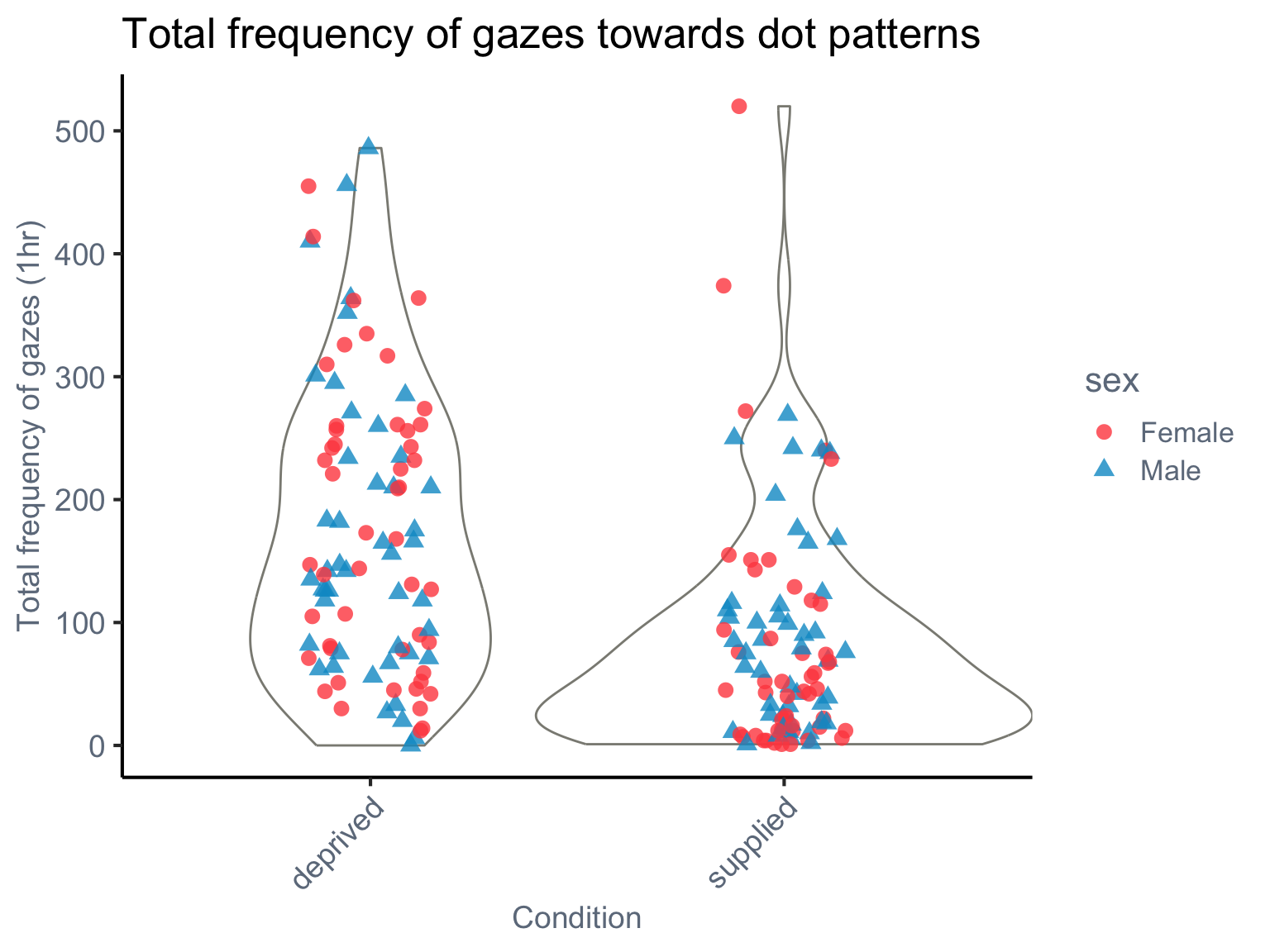
To avoid repeating the structure of the previous example, we now take a more realistic modeling approach by incorporating phylogenetic non-independence as a random effect. The response variable, frequency, is a count variable, which supports the use of Poisson or Negative Binomial distributions. However, as visualised in the plots below, there is substantial between-species variation—both in mean gaze frequency and in the degree of within-species variability.
To better capture this structure, we include phylogeny as a random effect, distinct from the previously used species effect. While species was treated as a simple categorical grouping factor, the phylogenetic random effect accounts for shared evolutionary history and allows for correlated responses among closely related species.
In the following sections, we will:
Include phylogeny as a random effect in the location and/or scale parts of the model.
Compare models with and without phylogenetic structure to evaluate whether accounting for evolutionary history improves model fit.
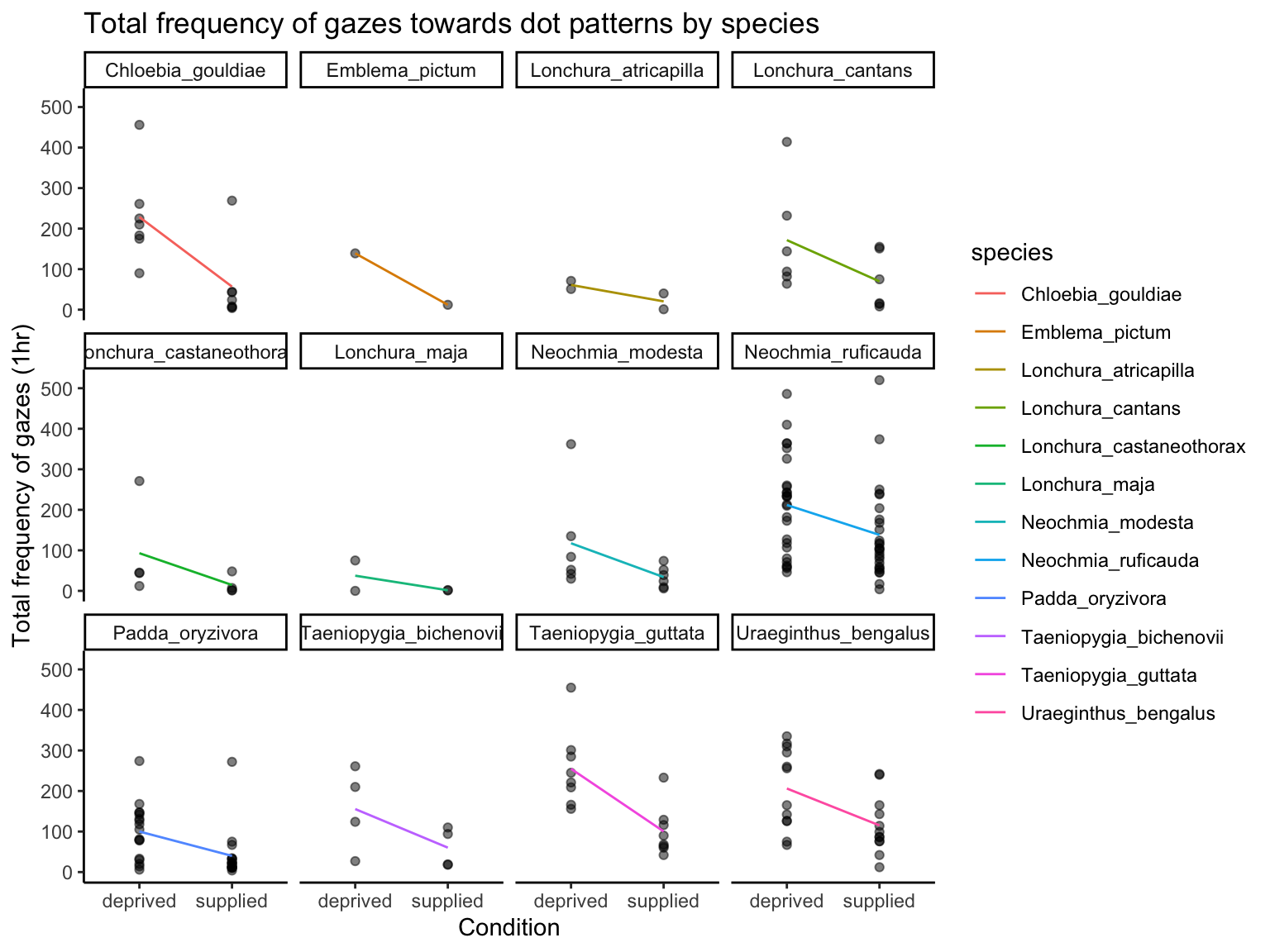
The violin plot by condition and sex shows that gaze frequency is generally higher in the food-deprived condition, with some individuals—especially females—showing very high values (over 500). The faceted line plot by species shows:
Consistent directional trends (e.g., reduced gazing in the supplied condition)
Species-specific differences in variance, suggesting possible heteroscedasticity
These patterns raise two important considerations:
Overdispersion is likely present, particularly in the deprived condition, where the spread of counts is large.
A phylogenetic effect may be at play, since species vary not only in their average gaze frequencies but also in how consistent individuals are within each species - possibly due to traits shaped by common ancestry.
dat_pref<-read.csv(here("data", "AM_preference.csv"), header =TRUE)dat_pref<-dat_pref%>%dplyr::select(-stripe, -full, -subset)%>%rename(frequency =dot)%>%mutate(species =phylo, across(c(condition, sex), as.factor))ggplot(dat_pref, aes(x =condition, y =frequency))+geom_violin(color ="#8B8B83", fill ="white", width =1.2, alpha =0.3)+geom_jitter(aes(shape =sex, color =sex), size =3, alpha =0.8, width =0.15, height =0)+labs( title ="Total frequency of gazes towards dot patterns", x ="Condition", y ="Total frequency of gazes (1hr)")+scale_shape_manual(values =c("M"=17, "F"=16), labels =c("M"="Male", "F"="Female"))+scale_color_manual(values =c("M"="#009ACD", "F"="#FF4D4D"), labels =c("M"="Male", "F"="Female"))+theme_classic(base_size =16)+theme( axis.text =element_text(color ="#6E7B8B", size =14), axis.title =element_text(color ="#6E7B8B", size =14), legend.title =element_text(color ="#6E7B8B"), legend.text =element_text(color ="#6E7B8B"), legend.position ="right", axis.text.x =element_text(angle =45, hjust =1))
ggplot(dat_pref, aes(x =dat_pref$condition, y =dat_pref$frequency))+geom_point(alpha =0.5)+labs( title ="Total frequency of gazes towards dot patterns by species", x ="Condition", y ="Total frequency of gazes (1hr)")+stat_summary(fun =mean, geom ="line", aes(group =species, color =species))+theme_classic()+facet_wrap(~species)
9.0.0.2 Begin with a simpler model and check residual diagnostics
From the previous analysis, we already know that a location-only model without phylogenetic effects does not adequately capture the structure of the data. However, here we re-examine this model before moving on.
model_0<-glmmTMB(frequency~1+condition+sex+(1|species)+(1|id), # location part (mean) data =dat_pref, family =nbinom2(link ="log"))
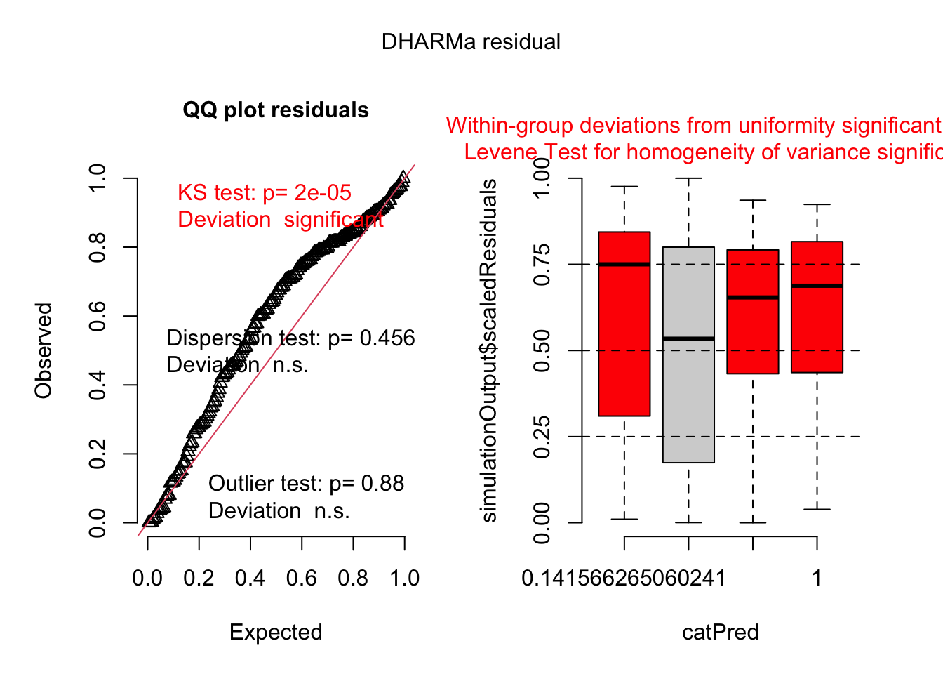
To evaluate model adequacy, we use the DHARMa package to simulate and visualise residuals. The plots allow us to assess residual uniformity, potential over- or underdispersion, outliers, and leverage.
# main diagnostic plotsmodel0_res<-simulateResiduals(model_0, plot =TRUE, seed =42)
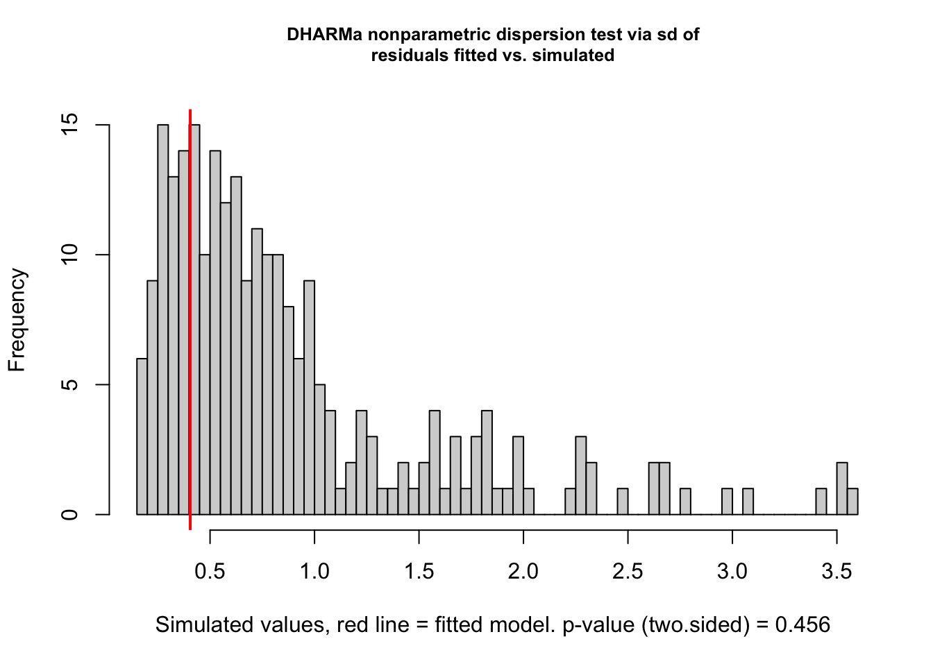
# formal test for over/underdispersiontestDispersion(model0_res)
    DHARMa nonparametric dispersion test via sd of residuals fitted vs.
    simulated

data:  simulationOutput
dispersion = 0.45606, p-value = 0.456
alternative hypothesis: two.sided
Although the dispersion test (p = 0.456) suggests no clear evidence of overdispersion based on the mean–variance relationship, the KS test indicates that the residuals deviate from a uniform distribution. These two tests assess different aspects of model adequacy: the dispersion test evaluates whether the variance is correctly specified as a function of the mean, while the KS test can detect broader misfits, such as unmodeled structure, zero inflation, or group-specific heteroscedasticity. Thus, even in the absence of overdispersion, the presence of non-uniform residuals supports the need for a more flexible model.
Since we have found the limitations of the model without phylogenetic effects, we now proceed to fit the same model using the brms package, this time including the phylogenetic effect as a random effect to account for the non-independence among species. Including both species and phylogeny as random effects allows us to distinguish between two sources of variation: the phylogenetic effect captures correlations arising from shared evolutionary history, whereas the species-level random intercept absorbs residual species-specific variation not accounted for by the tree—such as ecological or methodological factors. Including both terms helps avoid underestimating heterogeneity at the species level and provides a more accurate partitioning of variance.
First, we run the same model as above, but using the brms package. Then, we will gradually increase the model complexity by adding phylogenetic effects and a scale part to the model.
formula_eg2.0<-bf(frequency~1+condition+sex+(1|species)+(1|id))prior_eg2.0<-default_prior(formula_eg2.0, data =dat_pref, family =negbinomial(link ="log"))model_eg2.0<-brm(formula_eg2.0, data =dat_pref, prior =prior_eg2.0, chains =2, iter =5000, warmup =3000, thin =1, family =negbinomial(link ="log"), save_pars =save_pars(all =TRUE)# control = list(adapt_delta = 0.95))
Then, we add the phylogenetic effect as a random effect to the model. This allows us to account for the non-independence among species due to shared evolutionary history.
tree<-read.nexus(here("data", "AM_est_tree.txt"))tree<-force.ultrametric(tree, method ="extend")# is.ultrametric(tree)tip<-c("Lonchura_cantans","Uraeginthus_bengalus","Neochmia_modesta","Lonchura_atricapilla","Padda_oryzivora","Taeniopygia_bichenovii","Emblema_pictum","Neochmia_ruficauda","Lonchura_maja","Taeniopygia_guttata","Chloebia_gouldiae","Lonchura_castaneothorax")tree<-KeepTip(tree, tip, preorder =TRUE, check =TRUE)# Create phylogenetic correlation matrixA<-ape::vcv.phylo(tree, corr =TRUE)# Specify the model formula (location-only)formula_eg2.1<-bf(frequency~1+condition+sex+(1|a|gr(phylo, cov =A))+# phylogenetic random effect(1|species)+# non-phylogenetic species-level random effect (ecological factors)(1|id)# individual-level random effect)prior_eg2.1<-brms::get_prior( formula =formula_eg2.1, data =dat_pref, data2 =list(A =A), family =negbinomial(link ="log"))model_eg2.1<-brm( formula =formula_eg2.1, data =dat_pref, data2 =list(A =A), chains =2, iter =12000, warmup =10000, thin =1, family =negbinomial(link ="log"), prior =prior_eg2.1, control =list(adapt_delta =0.95), save_pars =save_pars(all =TRUE))
 Family: negbinomial
  Links: mu = log
Formula: frequency ~ condition + sex + (1 | species) + (1 | id)
   Data: dat_pref (Number of observations: 190)
  Draws: 2 chains, each with iter = 5000; warmup = 3000; thin = 1;
         total post-warmup draws = 4000

Multilevel Hyperparameters:
~id (Number of levels: 95)
              Estimate Est.Error l-95% CI u-95% CI Rhat Bulk_ESS Tail_ESS
sd(Intercept)     0.37      0.12     0.10     0.58 1.00      742      638

~species (Number of levels: 12)
              Estimate Est.Error l-95% CI u-95% CI Rhat Bulk_ESS Tail_ESS
sd(Intercept)     0.74      0.24     0.39     1.31 1.00     1464     2169

Regression Coefficients:
                  Estimate Est.Error l-95% CI u-95% CI Rhat Bulk_ESS Tail_ESS
Intercept             4.84      0.27     4.28     5.35 1.00     1827     2167
conditionsupplied    -0.92      0.13    -1.17    -0.68 1.00     5979     2911
sexM                 -0.07      0.15    -0.37     0.23 1.00     5172     2848

Further Distributional Parameters:
      Estimate Est.Error l-95% CI u-95% CI Rhat Bulk_ESS Tail_ESS
shape     1.71      0.23     1.31     2.22 1.00     1311     2090

Draws were sampled using sampling(NUTS). For each parameter, Bulk_ESS
and Tail_ESS are effective sample size measures, and Rhat is the potential
scale reduction factor on split chains (at convergence, Rhat = 1).
 Family: negbinomial
  Links: mu = log
Formula: frequency ~ condition + sex + (1 | a | gr(phylo, cov = A)) + (1 | species) + (1 | id)
   Data: dat_pref (Number of observations: 190)
  Draws: 2 chains, each with iter = 12000; warmup = 10000; thin = 1;
         total post-warmup draws = 4000

Multilevel Hyperparameters:
~id (Number of levels: 95)
              Estimate Est.Error l-95% CI u-95% CI Rhat Bulk_ESS Tail_ESS
sd(Intercept)     0.37      0.12     0.07     0.58 1.00      558      437

~phylo (Number of levels: 12)
              Estimate Est.Error l-95% CI u-95% CI Rhat Bulk_ESS Tail_ESS
sd(Intercept)     0.65      0.30     0.10     1.34 1.00     1035     1075

~species (Number of levels: 12)
              Estimate Est.Error l-95% CI u-95% CI Rhat Bulk_ESS Tail_ESS
sd(Intercept)     0.38      0.28     0.02     1.01 1.00      883     1654

Regression Coefficients:
                  Estimate Est.Error l-95% CI u-95% CI Rhat Bulk_ESS Tail_ESS
Intercept             4.99      0.38     4.23     5.74 1.00     1561     1724
conditionsupplied    -0.92      0.12    -1.16    -0.69 1.00     3485     2979
sexM                 -0.07      0.14    -0.35     0.21 1.00     2971     2976

Further Distributional Parameters:
      Estimate Est.Error l-95% CI u-95% CI Rhat Bulk_ESS Tail_ESS
shape     1.72      0.24     1.31     2.23 1.00     1121     1981

Draws were sampled using sampling(NUTS). For each parameter, Bulk_ESS
and Tail_ESS are effective sample size measures, and Rhat is the potential
scale reduction factor on split chains (at convergence, Rhat = 1).
9.0.0.3 Gradually increase model complexity
In the previous model, variation in individual gaze frequency was modeled assuming a constant dispersion parameter across all groups. However, visual inspection of the raw data suggests heteroscedasticity (i.e., group-specific variance). To accommodate this, we now fit a location-scale model where the shape (dispersion) parameter is allowed to vary by condition and sex.
This model helps capture structured variability in the data and may reveal whether the precision (or variability) of gaze frequency differs systematically between experimental groups.
# Specify the model formula (location-scale) - the scale part does not include random effectsformula_eg2.2<-bf(frequency~1+condition+sex+(1|a|gr(phylo, cov =A))+(1|species)+(1|id), shape~1+condition+sex)prior_eg2.2<-brms::get_prior( formula =formula_eg2.2, data =dat_pref, data2 =list(A =A), family =negbinomial(link ="log", link_shape ="log"))model_eg2.2<-brm( formula =formula_eg2.2, data =dat_pref, data2 =list(A =A), chains =2, iter =12000, warmup =10000, thin =1, family =negbinomial(link ="log", link_shape ="log"), prior =prior_eg2.2, control =list(adapt_delta =0.95), save_pars =save_pars(all =TRUE))
# specify the model formula (location-scale)## the scale part includes phylogenetic random effects and individual-level random effectsformula_eg2.3<-bf(frequency~1+condition+sex+(1|a|gr(phylo, cov =A))+# phylogenetic random effect(1|species)+# non-phylogenetic species-level random effect (ecological factors)(1|id), # individual-level random effectshape~1+condition+sex+(1|a|gr(phylo, cov =A))+(1|species)+(1|id))prior_eg2.3<-brms::get_prior( formula =formula_eg2.3, data =dat_pref, data2 =list(A =A), family =negbinomial(link ="log", link_shape ="log"))model_eg2.3<-brm( formula =formula_eg2.3, data =dat_pref, data2 =list(A =A), chains =2, iter =12000, warmup =10000, thin =1, family =negbinomial(link ="log", link_shape ="log"), prior =prior_eg2.3, control =list(adapt_delta =0.95), save_pars =save_pars(all =TRUE))summary(model_eg2.3)
 Family: negbinomial
  Links: mu = log; shape = log
Formula: frequency ~ condition + sex + (1 | a | gr(phylo, cov = A)) + (1 | species) + (1 | id)
         shape ~ condition + sex
   Data: dat_pref (Number of observations: 190)
  Draws: 2 chains, each with iter = 12000; warmup = 10000; thin = 1;
         total post-warmup draws = 4000

Multilevel Hyperparameters:
~id (Number of levels: 95)
              Estimate Est.Error l-95% CI u-95% CI Rhat Bulk_ESS Tail_ESS
sd(Intercept)     0.36      0.13     0.06     0.58 1.01      477      626

~phylo (Number of levels: 12)
              Estimate Est.Error l-95% CI u-95% CI Rhat Bulk_ESS Tail_ESS
sd(Intercept)     0.62      0.29     0.10     1.30 1.00      876      780

~species (Number of levels: 12)
              Estimate Est.Error l-95% CI u-95% CI Rhat Bulk_ESS Tail_ESS
sd(Intercept)     0.33      0.24     0.01     0.90 1.00      767     1774

Regression Coefficients:
                        Estimate Est.Error l-95% CI u-95% CI Rhat Bulk_ESS
Intercept                   5.02      0.36     4.31     5.77 1.00     1949
shape_Intercept             0.86      0.26     0.38     1.40 1.00     1139
conditionsupplied          -0.84      0.12    -1.08    -0.61 1.00     5098
sexM                       -0.11      0.14    -0.39     0.17 1.00     3822
shape_conditionsupplied    -0.68      0.26    -1.23    -0.19 1.00     2095
shape_sexM                  0.12      0.24    -0.35     0.58 1.00     4398
                        Tail_ESS
Intercept                   2101
shape_Intercept             2335
conditionsupplied           3033
sexM                        2663
shape_conditionsupplied     2510
shape_sexM                  3318

Draws were sampled using sampling(NUTS). For each parameter, Bulk_ESS
and Tail_ESS are effective sample size measures, and Rhat is the potential
scale reduction factor on split chains (at convergence, Rhat = 1).
 Family: negbinomial
  Links: mu = log; shape = log
Formula: frequency ~ condition + sex + (1 | a | gr(phylo, cov = A)) + (1 | species) + (1 | id)
         shape ~ condition + sex + (1 | a | gr(phylo, cov = A)) + (1 | species) + (1 | id)
   Data: dat_pref (Number of observations: 190)
  Draws: 2 chains, each with iter = 12000; warmup = 10000; thin = 1;
         total post-warmup draws = 4000

Multilevel Hyperparameters:
~id (Number of levels: 95)
                    Estimate Est.Error l-95% CI u-95% CI Rhat Bulk_ESS Tail_ESS
sd(Intercept)           0.31      0.11     0.05     0.51 1.00      533      501
sd(shape_Intercept)     0.21      0.15     0.01     0.57 1.00     1125     1444

~phylo (Number of levels: 12)
                               Estimate Est.Error l-95% CI u-95% CI Rhat
sd(Intercept)                      0.49      0.25     0.05     1.04 1.00
sd(shape_Intercept)                0.74      0.38     0.09     1.63 1.00
cor(Intercept,shape_Intercept)     0.51      0.44    -0.64     0.99 1.00
                               Bulk_ESS Tail_ESS
sd(Intercept)                       759      670
sd(shape_Intercept)                1060      983
cor(Intercept,shape_Intercept)      854     1112

~species (Number of levels: 12)
                    Estimate Est.Error l-95% CI u-95% CI Rhat Bulk_ESS Tail_ESS
sd(Intercept)           0.27      0.20     0.01     0.74 1.00      833     1644
sd(shape_Intercept)     0.46      0.33     0.02     1.24 1.00      826     1519

Regression Coefficients:
                        Estimate Est.Error l-95% CI u-95% CI Rhat Bulk_ESS
Intercept                   5.07      0.30     4.46     5.65 1.00     1501
shape_Intercept             0.85      0.50    -0.16     1.84 1.00     1384
conditionsupplied          -0.77      0.11    -0.99    -0.54 1.00     3387
sexM                       -0.15      0.13    -0.40     0.11 1.00     2191
shape_conditionsupplied    -0.70      0.26    -1.22    -0.21 1.00     2251
shape_sexM                  0.12      0.26    -0.40     0.62 1.00     2814
                        Tail_ESS
Intercept                   2213
shape_Intercept             1884
conditionsupplied           2669
sexM                        2480
shape_conditionsupplied     2726
shape_sexM                  2867

Draws were sampled using sampling(NUTS). For each parameter, Bulk_ESS
and Tail_ESS are effective sample size measures, and Rhat is the potential
scale reduction factor on split chains (at convergence, Rhat = 1).
9.0.0.4 Compare models using information criteria
To assess whether model fit improves with increased complexity, we compare models using Leave-One-Out Cross-Validation (LOO).
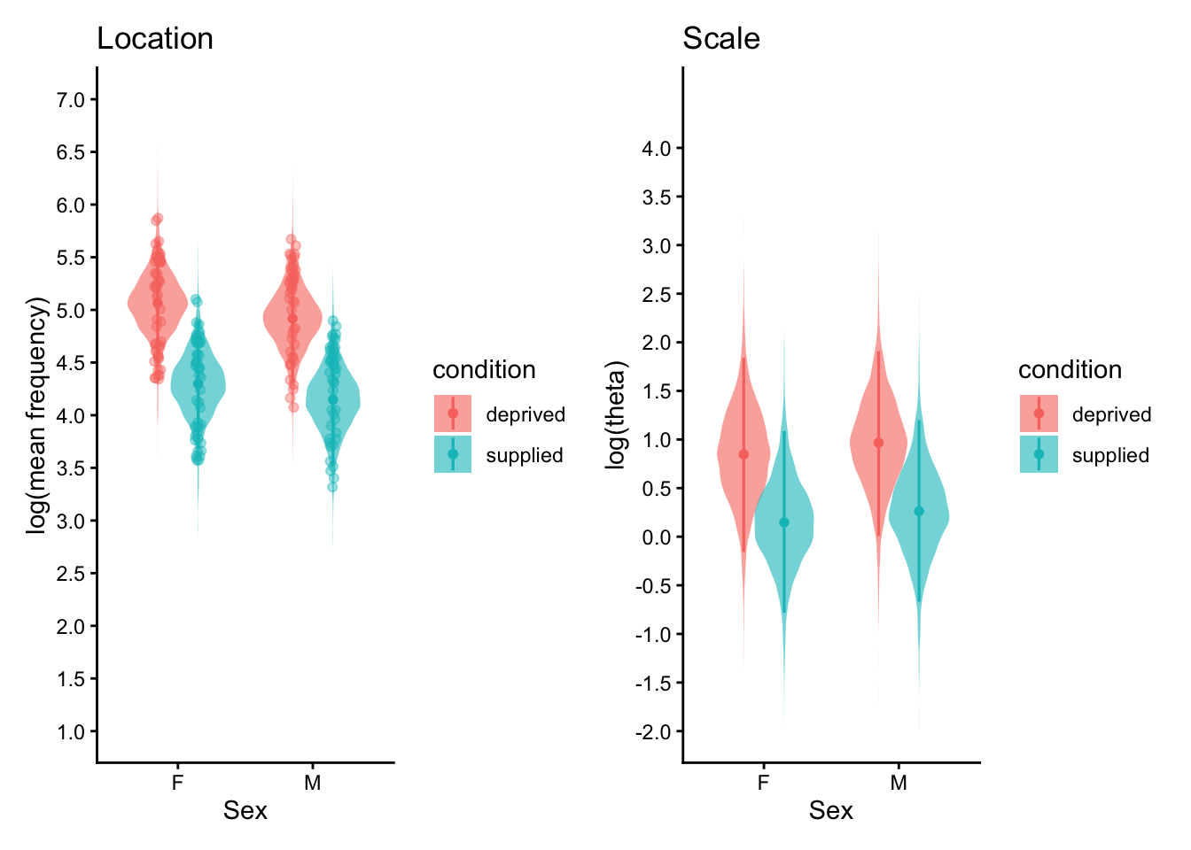
Model eg2.3, which includes both phylogenetic and species-level effects on the location and scale parts, performs best (highest elpd).
ELPD stands for Expected Log Predictive Density. It is a measure of out-of-sample predictive accuracy—that is, how well a model is expected to predict new, unseen data. - It is used in Bayesian model comparison, especially when using LOO-CV (Leave-One-Out Cross-Validation). - Higher ELPD means better predictive performance. - It is calculated by taking the log-likelihood of each observation, averaged over posterior draws, and then summed over all observations. - It rewards models that fit the data well without over-fitting.
 Family: negbinomial
  Links: mu = log; shape = log
Formula: frequency ~ condition + sex + (1 | a | gr(phylo, cov = A)) + (1 | species) + (1 | id)
         shape ~ condition + sex + (1 | a | gr(phylo, cov = A)) + (1 | species) + (1 | id)
   Data: dat_pref (Number of observations: 190)
  Draws: 2 chains, each with iter = 12000; warmup = 10000; thin = 1;
         total post-warmup draws = 4000

Multilevel Hyperparameters:
~id (Number of levels: 95)
                    Estimate Est.Error l-95% CI u-95% CI Rhat Bulk_ESS Tail_ESS
sd(Intercept)           0.31      0.11     0.05     0.51 1.00      533      501
sd(shape_Intercept)     0.21      0.15     0.01     0.57 1.00     1125     1444

~phylo (Number of levels: 12)
                               Estimate Est.Error l-95% CI u-95% CI Rhat
sd(Intercept)                      0.49      0.25     0.05     1.04 1.00
sd(shape_Intercept)                0.74      0.38     0.09     1.63 1.00
cor(Intercept,shape_Intercept)     0.51      0.44    -0.64     0.99 1.00
                               Bulk_ESS Tail_ESS
sd(Intercept)                       759      670
sd(shape_Intercept)                1060      983
cor(Intercept,shape_Intercept)      854     1112

~species (Number of levels: 12)
                    Estimate Est.Error l-95% CI u-95% CI Rhat Bulk_ESS Tail_ESS
sd(Intercept)           0.27      0.20     0.01     0.74 1.00      833     1644
sd(shape_Intercept)     0.46      0.33     0.02     1.24 1.00      826     1519

Regression Coefficients:
                        Estimate Est.Error l-95% CI u-95% CI Rhat Bulk_ESS
Intercept                   5.07      0.30     4.46     5.65 1.00     1501
shape_Intercept             0.85      0.50    -0.16     1.84 1.00     1384
conditionsupplied          -0.77      0.11    -0.99    -0.54 1.00     3387
sexM                       -0.15      0.13    -0.40     0.11 1.00     2191
shape_conditionsupplied    -0.70      0.26    -1.22    -0.21 1.00     2251
shape_sexM                  0.12      0.26    -0.40     0.62 1.00     2814
                        Tail_ESS
Intercept                   2213
shape_Intercept             1884
conditionsupplied           2669
sexM                        2480
shape_conditionsupplied     2726
shape_sexM                  2867

Draws were sampled using sampling(NUTS). For each parameter, Bulk_ESS
and Tail_ESS are effective sample size measures, and Rhat is the potential
scale reduction factor on split chains (at convergence, Rhat = 1).
Accounting for phylogeny captures much of the between-species structure, it highlights evolutionary constraints or shared ecological traits. The remaining species-specific variance suggests additional factors (e.g., experimental nuances) not captured by the tree alone.
Source Code
---title: "Model Selection (Example 2)"---```{r}#| label: load_packages#| echo: false# Load required packagespacman::p_load(## data manipulation dplyr, tibble, tidyverse, broom, broom.mixed,## model fitting ape, arm, brms, broom.mixed, cmdstanr, emmeans, glmmTMB, MASS, phytools, rstan, TreeTools,## model checking and evaluation DHARMa, loo, MuMIn, parallel,## visualisation bayesplot, ggplot2, patchwork, tidybayes,## reporting and utilities gt, here, kableExtra, knitr)```We revisit the dataset on Estrildid finches to examine how food supplementation affects gaze frequency toward dot patterns (as introduced in `Beyond Gaussian 1` section).To avoid repeating the structure of the previous example, we now take a more realistic modeling approach by incorporating phylogenetic non-independence as a random effect. The response variable, frequency, is a count variable, which supports the use of Poisson or Negative Binomial distributions. However, as visualised in the plots below, there is substantial between-species variation—both in mean gaze frequency and in the degree of within-species variability.To better capture this structure, we include phylogeny as a random effect, distinct from the previously used species effect. While species was treated as a simple categorical grouping factor, the phylogenetic random effect accounts for shared evolutionary history and allows for correlated responses among closely related species.In the following sections, we will:- Include phylogeny as a random effect in the location and/or scale parts of the model.- Compare models with and without phylogenetic structure to evaluate whether accounting for evolutionary history improves model fit.::: panel-tabset### Step 1#### Identify data type and plot raw dataThe violin plot by condition and sex shows that gaze frequency is generally higher in the food-deprived condition, with some individuals—especially females—showing very high values (over 500). The faceted line plot by species shows: - Consistent directional trends (e.g., reduced gazing in the supplied condition)- Species-specific differences in variance, suggesting possible heteroscedasticityThese patterns raise two important considerations: 1. Overdispersion is likely present, particularly in the deprived condition, where the spread of counts is large. 2. A phylogenetic effect may be at play, since species vary not only in their average gaze frequencies but also in how consistent individuals are within each species - possibly due to traits shaped by common ancestry.```{r}#| label: identify_data_type - eg2#| fig-width: 8#| fig-height: 6dat_pref <-read.csv(here("data", "AM_preference.csv"), header =TRUE)dat_pref <- dat_pref %>% dplyr::select(-stripe, -full, -subset) %>%rename(frequency = dot) %>%mutate(species = phylo, across(c(condition, sex), as.factor))ggplot(dat_pref, aes(x = condition,y = frequency)) +geom_violin(color ="#8B8B83", fill ="white",width =1.2, alpha =0.3) +geom_jitter(aes(shape = sex, color = sex),size =3, alpha =0.8,width =0.15, height =0) +labs(title ="Total frequency of gazes towards dot patterns",x ="Condition",y ="Total frequency of gazes (1hr)" ) +scale_shape_manual(values =c("M"=17, "F"=16),labels =c("M"="Male", "F"="Female")) +scale_color_manual(values =c("M"="#009ACD", "F"="#FF4D4D"),labels =c("M"="Male", "F"="Female")) +theme_classic(base_size =16) +theme(axis.text =element_text(color ="#6E7B8B", size =14),axis.title =element_text(color ="#6E7B8B", size =14),legend.title =element_text(color ="#6E7B8B"),legend.text =element_text(color ="#6E7B8B"),legend.position ="right",axis.text.x =element_text(angle =45, hjust =1) )ggplot(dat_pref, aes(x = dat_pref$condition, y = dat_pref$frequency)) +geom_point(alpha =0.5) +labs(title ="Total frequency of gazes towards dot patterns by species",x ="Condition",y ="Total frequency of gazes (1hr)" ) +stat_summary(fun = mean, geom ="line", aes(group = species, color = species)) +theme_classic() +facet_wrap(~ species)```### Steps 2 and 3#### Begin with a simpler model and check residual diagnosticsFrom the previous analysis, we already know that a location-only model without phylogenetic effects does not adequately capture the structure of the data. However, here we re-examine this model before moving on.```{r}#| label: model_fitting - eg2model_0 <-glmmTMB( frequency ~1+ condition + sex + (1| species) + (1| id), # location part (mean)data = dat_pref,family =nbinom2(link ="log"))```To evaluate model adequacy, we use the `DHARMa` package to simulate and visualise residuals. The plots allow us to assess residual uniformity, potential over- or underdispersion, outliers, and leverage.```{r}#| label: residual_diagnostics - eg2# main diagnostic plotsmodel0_res <-simulateResiduals(model_0, plot =TRUE, seed =42)# formal test for over/underdispersiontestDispersion(model0_res) ```Although the dispersion test (`p = 0.456`) suggests no clear evidence of overdispersion based on the mean–variance relationship, the KS test indicates that the residuals deviate from a uniform distribution. These two tests assess different aspects of model adequacy: the dispersion test evaluates whether the variance is correctly specified as a function of the mean, while the KS test can detect broader misfits, such as unmodeled structure, zero inflation, or group-specific heteroscedasticity. Thus, even in the absence of overdispersion, the presence of non-uniform residuals supports the need for a more flexible model.Since we have found the limitations of the model without phylogenetic effects, we now proceed to fit the same model using the `brms` package, this time including the phylogenetic effect as a random effect to account for the non-independence among species. Including both species and phylogeny as random effects allows us to distinguish between two sources of variation: the phylogenetic effect captures correlations arising from shared evolutionary history, whereas the species-level random intercept absorbs residual species-specific variation not accounted for by the tree—such as ecological or methodological factors. Including both terms helps avoid underestimating heterogeneity at the species level and provides a more accurate partitioning of variance.First, we run the same model as above, but using the `brms` package. Then, we will gradually increase the model complexity by adding phylogenetic effects and a scale part to the model.```{r}#| label: model_fitting1 - eg2#| eval: falseformula_eg2.0<-bf( frequency ~1+ condition + sex + (1| species) + (1| id))prior_eg2.0<-default_prior(formula_eg2.0, data = dat_pref, family =negbinomial(link ="log"))model_eg2.0<-brm(formula_eg2.0, data = dat_pref, prior = prior_eg2.0,chains =2, iter =5000, warmup =3000,thin =1,family =negbinomial(link ="log"),save_pars =save_pars(all =TRUE)# control = list(adapt_delta = 0.95))```Then, we add the phylogenetic effect as a random effect to the model. This allows us to account for the non-independence among species due to shared evolutionary history.```{r}#| label: model_fitting2 - eg2#| eval: falsetree <-read.nexus(here("data", "AM_est_tree.txt"))tree <-force.ultrametric(tree, method ="extend")# is.ultrametric(tree)tip <-c("Lonchura_cantans","Uraeginthus_bengalus","Neochmia_modesta","Lonchura_atricapilla","Padda_oryzivora","Taeniopygia_bichenovii","Emblema_pictum","Neochmia_ruficauda","Lonchura_maja","Taeniopygia_guttata","Chloebia_gouldiae","Lonchura_castaneothorax")tree <-KeepTip(tree, tip, preorder =TRUE, check =TRUE)# Create phylogenetic correlation matrixA <- ape::vcv.phylo(tree, corr =TRUE)# Specify the model formula (location-only)formula_eg2.1<-bf( frequency ~1+ condition + sex + (1| a |gr(phylo, cov = A)) +# phylogenetic random effect (1| species) +# non-phylogenetic species-level random effect (ecological factors) (1| id) # individual-level random effect)prior_eg2.1<- brms::get_prior(formula = formula_eg2.1, data = dat_pref, data2 =list(A = A),family =negbinomial(link ="log"))model_eg2.1<-brm(formula = formula_eg2.1, data = dat_pref, data2 =list(A = A),chains =2, iter =12000, warmup =10000,thin =1,family =negbinomial(link ="log"),prior = prior_eg2.1,control =list(adapt_delta =0.95),save_pars =save_pars(all =TRUE))``````{r}#| echo: falsemodel_eg2.0<-readRDS(here("Rdata", "model_eg2.0.rds"))summary(model_eg2.0)model_eg2.1<-readRDS(here("Rdata", "model_eg2.1.rds"))summary(model_eg2.1)```### Step 4#### Gradually increase model complexityIn the previous model, variation in individual gaze frequency was modeled assuming a constant dispersion parameter across all groups. However, visual inspection of the raw data suggests heteroscedasticity (i.e., group-specific variance). To accommodate this, we now fit a location-scale model where the shape (dispersion) parameter is allowed to vary by condition and sex.This model helps capture structured variability in the data and may reveal whether the precision (or variability) of gaze frequency differs systematically between experimental groups.```{r}#| eval: false# Specify the model formula (location-scale) - the scale part does not include random effectsformula_eg2.2<-bf( frequency ~1+ condition + sex + (1| a |gr(phylo, cov = A)) + (1| species) + (1| id), shape ~1+ condition + sex)prior_eg2.2<- brms::get_prior(formula = formula_eg2.2, data = dat_pref, data2 =list(A = A),family =negbinomial(link ="log", link_shape ="log"))model_eg2.2<-brm(formula = formula_eg2.2, data = dat_pref, data2 =list(A = A),chains =2, iter =12000, warmup =10000,thin =1,family =negbinomial(link ="log", link_shape ="log"),prior = prior_eg2.2,control =list(adapt_delta =0.95),save_pars =save_pars(all =TRUE))``````{r}#| eval: false# specify the model formula (location-scale)## the scale part includes phylogenetic random effects and individual-level random effectsformula_eg2.3<-bf( frequency ~1+ condition + sex + (1|a|gr(phylo, cov = A)) +# phylogenetic random effect (1| species) +# non-phylogenetic species-level random effect (ecological factors) (1| id), # individual-level random effectshape ~1+ condition + sex + (1|a|gr(phylo, cov = A)) + (1| species) + (1| id) )prior_eg2.3<- brms::get_prior(formula = formula_eg2.3, data = dat_pref, data2 =list(A = A),family =negbinomial(link ="log", link_shape ="log"))model_eg2.3<-brm(formula = formula_eg2.3, data = dat_pref, data2 =list(A = A),chains =2, iter =12000, warmup =10000,thin =1,family =negbinomial(link ="log", link_shape ="log"),prior = prior_eg2.3,control =list(adapt_delta =0.95),save_pars =save_pars(all =TRUE))summary(model_eg2.3)``````{r}#| echo: falsemodel_eg2.2<-readRDS(here("Rdata", "model_eg2.2.rds"))summary(model_eg2.2)model_eg2.3<-readRDS(here("Rdata", "model_eg2.3.rds"))summary(model_eg2.3)```### Step 5#### Compare models using information criteriaTo assess whether model fit improves with increased complexity, we compare models using Leave-One-Out Cross-Validation (LOO).```{r}#| eval: falseoptions(future.globals.maxSize =2*1024^3)loo_eg2.0<- loo::loo(model_eg2.0, moment_match =TRUE,reloo =TRUE, cores =2)loo_eg2.1<- loo::loo(model_eg2.1, moment_match =TRUE, reloo =TRUE, cores =2)loo_eg2.2<- loo::loo(model_eg2.2, moment_match =TRUE,reloo =TRUE, cores =2)loo_eg2.3<- loo::loo(model_eg2.3, moment_match =TRUE,reloo =TRUE, cores =2)fc_eg2 <- loo::loo_compare(loo_eg2.0, loo_eg2.1, loo_eg2.2, loo_eg2.3)print(fc_eg2)# elpd_diff se_diff# model_eg2.3 0.0 0.0 # model_eg2.1 -11.5 4.5 # model_eg2.2 -11.7 5.3 # model_eg2.0 -13.5 4.9 summary(model_eg2.3)```Model eg2.3, which includes both phylogenetic and species-level effects on the location and scale parts, performs best (highest elpd).ELPD stands for Expected Log Predictive Density. It is a measure of out-of-sample predictive accuracy—that is, how well a model is expected to predict new, unseen data. - It is used in Bayesian model comparison, especially when using LOO-CV (Leave-One-Out Cross-Validation). - Higher ELPD means better predictive performance. - It is calculated by taking the log-likelihood of each observation, averaged over posterior draws, and then summed over all observations. - It rewards models that fit the data well without over-fitting.```{r}#| echo: falsemodel_eg2.3<-readRDS(here("Rdata", "model_eg2.3.rds"))summary(model_eg2.3)# Create a grid of predictor values for posterior distributionsnd <- tidyr::expand_grid(condition =levels(dat_pref$condition),sex =levels(dat_pref$sex))# Get posterior draws for mu and shape and reshape the datadraws_link <- tidybayes::linpred_draws( model_eg2.3, newdata = nd, re_formula =NA, dpar =TRUE) %>%transmute( sex, condition, .draw,log_mu = mu,log_theta = shape ) %>% tidyr::pivot_longer(cols =c(log_mu, log_theta), names_to ="parameter", values_to ="value" )# Get the posterior median of the linear predictor for each observationpred_obs <-add_linpred_draws(newdata = dat_pref, # Use the original data hereobject = model_eg2.3,dpar ="mu",re_formula =NULL# Include group-level effects for specific predictions ) %>%group_by(.row, condition, sex) %>%# .row is added by add_linpred_drawssummarise(predicted_logmu =median(.linpred), # Calculate the posterior median.groups ="drop" )# Create the plot for the Location parameter (mu) with predicted pointsp_loc <- draws_link %>%filter(parameter =="log_mu") %>%ggplot(aes(x = sex, y = value, fill = condition)) +geom_violin(width =0.9, trim =FALSE, alpha =0.6,color =NA, position =position_dodge(0.6) ) +stat_pointinterval(aes(color = condition),position =position_dodge(width =0.6),.width =0.95, size =0.8 ) +# Add the new layer for predicted data pointsgeom_point(data = pred_obs,aes(y = predicted_logmu, color = condition), # y-aesthetic is the predicted valueposition =position_jitterdodge(dodge.width =0.6, # Must match the dodge width abovejitter.width =0.1 ),alpha =0.4,size =1.5 ) +labs(title ="Location", x ="Sex", y ="log(mean frequency)" ) +scale_y_continuous(limits =c(1.0, 7.0), breaks =seq(1.0, 7.0, by =0.5)) +theme_classic() +theme(legend.position ="right")# Create the plot for the Scale parameter (shape)p_scl <- draws_link %>%filter(parameter =="log_theta") %>%ggplot(aes(x = sex, y = value, fill = condition)) +geom_violin(width =0.9, trim =FALSE, alpha =0.6,color =NA, position =position_dodge(0.6) ) +stat_pointinterval(aes(color = condition),position =position_dodge(width =0.6),.width =0.95, size =0.8 ) +labs(title ="Scale", x ="Sex", y ="log(theta)" ) +scale_y_continuous(limits =c(-2.0, 4.5), breaks =seq(-2.0, 4.0, by =0.5)) +theme_classic() +theme(legend.position ="right")p_loc + p_scl```Accounting for phylogeny captures much of the between-species structure, it highlights evolutionary constraints or shared ecological traits. The remaining species-specific variance suggests additional factors (e.g., experimental nuances) not captured by the tree alone.:::